Database Reference
In-Depth Information
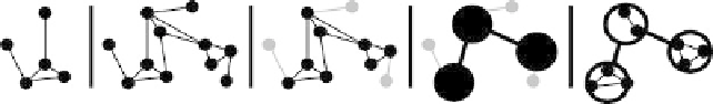
Fig. 3.3 Social network visualization possibilities
l
Find faster methods
l
Find better visualization techniques
l
Apply some simplification, which will allow us to maintain good overview of
network
l
Specify our interests more precisely and use computer algorithms to find impor-
tant parts
Finding faster methods is always a possibility, but we will surely reach a limit. In
this situation, more processed data means also more data for visualization (see first
two parts of Fig.
3.3
). Here, we will reach the limits of a particular visualization
technique, therefore we should think of a better visualization technique. A common
approach is to use another dimension (switching from 2D to 3D or using animation
rather a static image) or another visualization attribute (coloring nodes, sizing nodes,
and edges). Some of these enhancements can be used only in some specific environ-
ments and are not suited, for example, to grayscale printers (third part of Fig.
3.3
). If
it is so complicated to display so much information at once, perhaps the data could be
simplified with only the important parts being displayed (fourth part of Fig.
3.3
).
Clearly, this leads to the omission of less important information, which is not always
a suitable option. We have to know what is important. In this case, we specify the
objective using a pattern and let the algorithm search for it. Identified patterns can be
highlighted in visualizations or presented separately (last part of Fig.
3.3
).
3.1.4 Social Networks Representation
Social networks are usually modeled using graphs (see Fig.
3.4
). Below we recall
some basic notions from the graph theory. On a graph, we can consider a tuple
G
¼ð
V
;
E
Þ
, where
V
is the list of nodes (
V
¼
{
A
,
B
,
C
,
D
}) and
E
is the list of
edges (
E
¼
{
e
1
,
e
2
,
e
3
,
e
4
,
e
5
}). An edge connects two nodes and more formally
can be expressed as a tuple (
e
1
¼h
).
It is natural to represent the social network data and their respective graphs using
matrices as they can be immediately used in further computations. Graphs can be
modeled using the incidence matrix (rows are vertices, columns are edges, and the
value denotes the relation of the given vertex to the given edge; see Fig.
3.4
). The
incidence matrix of a directed graph usually contains values
A
;
B
i
1 (the edge starts
from the node), 0 (the node is not related to the edge), and 1 (the edge ends in the
node). Another form of a modeling graph is the adjacency matrix which represents
the relation between two nodes. Later in the text we will use this type of matrix.
Search WWH ::

Custom Search