Information Technology Reference
In-Depth Information
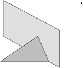
Epipolar plane
Π
e
M
l
m
l
m
m
m
e
e
C
C
right epipolar line
left epipolar line
Fig. 2
Epipolar geometry
and the point
C
projects to the point
e
in the left image (see Fig. 2). The two points
e
and
e
are the
epipoles
and the lines through
e
and
e
are the
epipolar lines
.Leta
space point
M
be projected on
m
and
m
respectively in the left and the right image
planes. The camera centers, the space point
M
and its image projections are coplanar
and form the plane
Π
e
, called
epipolar plane
. The projections of this plane into the
left and the right image are respectively the epipolar lines
l
m
and
l
m
. The epipolar
constraint states that the optical ray passing through
m
and
M
is mapped into the
corresponding epipolar line
l
m
in the right image plane and therefore that
m
must
lie on
l
m
. Reciprocally,
m
necessarily lies on the homologous epipolar line
l
m
which
represents the projection of the optical ray of
m
onto the left image plane. In terms
of a stereo correspondence algorithm, due to this epipolar constraint, the search of
corresponding points
m
and
m
does not need to cover the entire image plane but
can be reduced to a 1D search along the epipolar lines.
2.2.2
Parallel Cameras Geometry
The parallel camera configuration uses two cameras with parallel optical axes. In
this configuration, the epipoles move to infinity and the epipolar lines coincide with
horizontal scanlines. The matching point of a pixel in one view can then be found
on the same scanline in the other view. In a general camera setup, a technique called
rectification [9] is used to adjust images so that they are re-projected onto a plane
parallel to the baseline, as in the case of a parallel camera setup.
Consider a point
M
in the 3-D world with coordinates (
X
,
Y
,
Z
),
Z
being the
distance between the point
M
and the common cameras plane. Let the coordinates
of points
m
and
m
, projections of
M
on the left and right image planes, be (
x
,
y
) and
(
x
,
y
), respectively. By applying Thales theorem in similar triangles of Fig. 3, we
can derive