Information Technology Reference
In-Depth Information
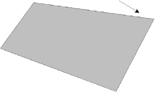
Fig. 3
Relative motion of a camera capturing a planar region
)=(
trace
(
R
)
cos
(
θ
−
1)
/
2
,
(6)
2
a
T
⎡
⎤
⎦
,
R
3
,
2
R
2
,
3
−
)=
1
⎣
R
1
,
3
−
R
3
,
1
sin
(
θ
R
2
,
1
−
R
1
,
2
where
R
i
,
j
is the element in the
i
-th row and
j
-th column of the estimated rotation
matrix
R
. Under constant velocity assumption, the decomposed motion parameters,
that is, the rotation angle
and the translation vector
t
, can be interpolated at a time
θ
instant
t
−
Δ
t
by a linear model:
b
=
θ
θΔ
t
,
t
b
=
t
Δ
t
.
(7)
In the general case, where the calibration matrices are known or can be estimated,
the backward homography matrix
P
t
−
Δ
t
b
is computed by plugging the interpolated
b
and
t
b
into Equations 5, 4 and 3, respectively. For the cases
where the calibration is not available, it is reasonable to assume that the amount of
change in focal length between
t
motion parameters
θ
K
t
). For the sake
of further simplicity, we shall use the small angle approximation of rotation:
1and
t
is negligible (i.e.
K
t
−
1
−
R
=
I
+
θ
[a]
x
.
(8)