Information Technology Reference
In-Depth Information
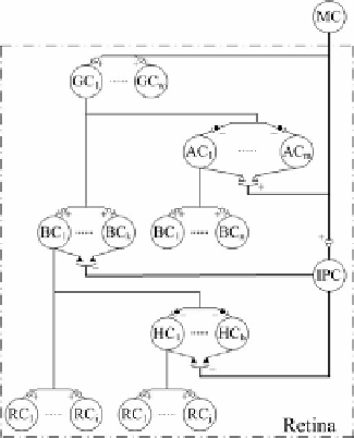
Fig. 1.
Neural circuit for dynamically adjusting
RF.
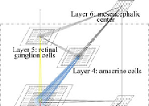
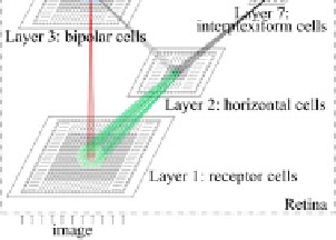
Fig. 2.
The multi-layer network model for
processing image.
3.2 Multi-layer Network Model for Image Processing
According to the above neural circuit for dynamically adjusting RF, we propose the
multi-layer network model for processing image shown in Fig. 2.
3.3 Numerical Calculation Model of GC's RF
The output of the second layer can be expressed as follow:
GC
(
X
,
Y
)
=
∑ ∑
W
⋅
RC
(
x
,
y
)
−
∑∑
W
⋅
RC
(
x
,
y
)
+
∑ ∑
W
⋅
RC
(
x
,
y
)
1
2
3
y
∈∈
S
x
S
y
∈∈
S
x
S
y
∈∈
S
x
S
1
1
2
2
3
3
(1)
2
2
2
2
2
2
(
x
−
x
)
+
(
y
−
y
)
(
x
−
x
)
+
(
y
−
y
)
(
x
−
x
)
+
(
y
−
y
)
−
0
0
−
0
0
−
0
0
2
1
2
2
2
3
σ
σ
σ
where
W
=
A
⋅
e
⋅
Δ
s
,
W
=
A
⋅
e
⋅
Δ
s
,
W
=
A
⋅
e
⋅
Δ
s
1
1
1
2
2
2
3
3
3
where, GC(X, Y) is the response of GC; RC(x, y) is image brightness projected onto
RC within RF; S
1
, S
2
and S
3
are CRF center, CRF surround and nCRF respectively;
W
1
, W
2
and W
3
are the weighting functions of the RCs within S
1
, S
2
and S
3
respectively; A
1
, A
2
and A
3
are the peak sensitivities of S
1
, S
2
and S
3
respectively; σ
1
,
σ
2
and σ
3
are the standard deviations of the three weighting functions respectively,
and 3σ
1
, 3σ
2
and 3σ
3
are the radii of S
1
, S
2
and S
3
respectively; ∆s
1
, ∆s
2
and ∆s
3
are
the bottom areas of the weights of the RCs in S
1
, S
2
and S
3
respectively; x and y are
position coordinates of RC; x
0
and y
0
are center coordinates of RF; X and Y are
position coordinates of retinal GC.
In our experiment, pictures are imaged on the central retina with the range of 0-10
degrees eccentricity.

Search WWH ::

Custom Search