Agriculture Reference
In-Depth Information
900
⎛
⎞
(
)
(
)
0.408
RG
−+γ
uee
−
⎜
⎟
n
⎝
⎠
2
s
a
T
+
273
ET
=
(2)
(
)
o
+γ
1
+
0.34
u
2
where: ET
o
= ET (mm day
-1
); ∆ = Slope of the vapor pressure curve (kPa°C
-1
); R
n
= Net
radiation at the crop surface (MJ m
-
2
day
-1
); G = Soil heat flux density (MJ m
-2
day
-1
);
a
= Mean air density at constant pressure (kg m
-3
); Cp = Specific heat at constant pressure
(MJ kg
-
1
°C
-1
); e
s
-e
a
= Vapor pressure deficit (kPa); e
s
= Saturation vapor pressure (kPa);
e
a
= Actual vapor pressure (kPa); r
a
= Aerodynamic resistance (s m
-1
); r
s
= The bulk sur-
face resistance (s m
-1
);
λ
= Latent heat of vaporization (MJ kg
-1
);
γ =
The psychrometric
constant (kPa°C
-1
).
Equation (1) applies specifi cally to a hypothetical reference crop with an assumed
crop height of 0.12 m, a fi xed surface resistance of 70 sec.m
1
and an albedo of 0.23.
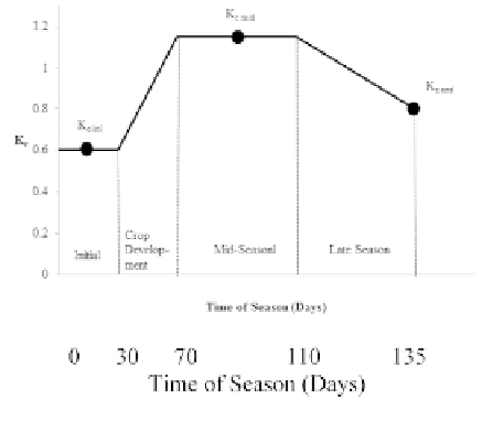
The crop coeffi cient, which changes throughout the crop season are shown in Fig. 1.
During the initial crop growth stage, the value of the crop coeffi cient is K
c ini
. During
the mid season the crop coeffi cient is K
c mid
, and at the end of the late season the crop
coeffi cient is K
c end
. The values of K
c ini
, K
c mid
and K
c end
can be obtained from published
tables [1].
ρ
FIGURE 1
Crop Coefficient Curve [1].
11.2.1
STEPS TO ESTIMATE IRRIGATION REQUIREMENT
Step 1.
Create an evapotranspiration crop coefficient curve for the crop. The
following link to the Food and Agriculture Organization (FAO) Document No.
56 [1] provides tables of crop stage growth (Table 11) and K
c
values (Table 12)
for a large number of crops: http://www.fao.org/docrep/X0490E/x0490e00.
htm. The K
c
curve should look like Fig. 1 when step 1 is finished. Note that
crop coefficient curves can also be created by using computer programs such
as PRET [8] or CropWat [3].


Search WWH ::

Custom Search