Information Technology Reference
In-Depth Information
(21)
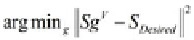
It is clear from (21) that the resulting current is desired to be a delta-like form
in the control angles
with some added noise. The scanning process is done
in the sense that the control angles
(
θ, ϕ
)
are going to be varied from 0 to
π
for
θ
and from 0 to 2
π
for
ϕ
. For each control angle set
(
θ, ϕ
)
,
I
out
is calculated by
first finding the optimal set of weight factors
g
V
. When the calculation is done
for all the angle sets, plotting
I
out
(
(
θ, ϕ
)
θ, ϕ
)
will show that the output will have its
maximum value at
which is the aim of the array. In this way by using
some kind of a maximum seeking circuit and after that determining at which
control angle set this maximum was found, the direction of arrival detection is
possible.
To transform
S
to
S
Desired
(
θ
s
,ϕ
s
)
the following problem must be solved for each
control angle set.
(22)
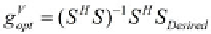
The above minimization statement can be easily solved for with respect to the
vector
g
V
by setting the vector to:
(23)
Note that the same analysis applies if more than one source is being detected.
3 Matlab Simulation Results
The theory presented in Section II is simulated in MATLAB. As mentioned
earlier 42 elements were used in the simulation. Each element has a dimension
of
L=2cm
and the frequency of reception is taken to be 500 kHz. The spacing
between the centers of the elements is
≈
4cm
. For an operating frequency of 500
kHz the electromagnetic properties of the human head in region 0-3 are as follows
(as given in [15]): region (0) has the free space permittivity and permeability;
region (1) has
ε
1
=38
.
87
0
,
μ
1
=
μ
0
&
σ
1
=1
.
88
S
/
m
;region(2)has
ε
2
=19
.
34
0
,
μ
2
=
5
S
/
m
.
The simulations in Figures 3-5 show how the output current
I
out
in (21) varies
with the angular parameters
θ
and
ϕ
. Note that all the simulations made are
for a radial distance of
r
(0)
=5cm
μ
0
&
σ
2
=0
.
59
S
/
m
; and region (3) has
ε
3
=51
.
8
0
,
μ
3
=
μ
0
&
σ
3
=1
.
from the center of the coordinate system as
showninFig.1.
It is clear from the figures that the beamforming technique is successful in
determining the direction of the source H-field
indicated by each figure.
The origin of the source clearly corresponds to the maximum value in the output
current at every case. For the case of Fig. 5b it is clear that the technique is
(
θ, ϕ
)

Search WWH ::

Custom Search