Geoscience Reference
In-Depth Information
t
(s)
t
(s)
0.
4
0.3
0.2
0.1
0
0
0.1
0.2
0.3
0.4
0
0
200
200
400
400
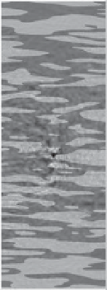
Figure 6.15
The propagating wave field
recorded at the seismic receivers in the
two boreholes located in the vicinity of
the scanning area. Similar seismograms
could be obtained by linear
superposition of seismograms generated
from individual locations in the
boreholes, after appropriate phase
delay corresponding to the desired
focusing point in the region
ℜ
.
600
600
800
800
1000
1000
× (m)
× (m)
× (m)
0
200
400
200
400
0
200
400
0
0
0
0
200
200
200
400
400
400
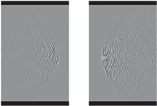
Figure 6.16
Seismic wave field obtained
by backpropagating the recorded seismic
signals into the medium in order to focus
seismic energy at the location of the
original scanning point (time reversal).
In this case, the seismograms do not
need to be delayed since they are
generated through modeling from the
desired focusing point.
600
600
600
800
800
800
1000
1000
1000
In the next section, the structural information con-
tained in this seismoelectric image is used to guide the
inversion of electrical resistivity data using current
sources and potential receivers located in the two wells.
in the previous section, we can proceed to the next step,
that is, to invert for the distribution of electrical conduc-
tivity in the medium using apparent resistivity data
acquired with a set of electrodes located in the two wells.
We show in this section that this method may improve
substantially the resolution of cross-well ERT.
6.3.2 Step 2: application of image-guided
inversion to ERT
In this section, we consider a set of electrodes located in
the two wells with a spacing of
L
=10 ms between the
electrodes. Using the map of electric potential defined
6.3.2.1 Edge detection
First, we filter the seismoelectric image to detect the
boundaries of
the different
formations. Among the