Geoscience Reference
In-Depth Information
Raw electrograms
60
40
20
1
2
3
4
5
6
7
8
9
10
11
12
13
14
15
16
17
18
19
20
21
22
23
24
25
26
27
28
29
30
31
32
0
−20
−40
−60
140
141
142
143
144
145
146
147
148
Time (s)
(a)
Detrended and synchronized electrograms
30
Injection
t
20
= 145.1 s
10
Preinjection
0
−10
−20
Injection
window
−30
140
141
142
143
144
145
146
147
148
Time (s)
(b)
Electrograms from 144.5 s to 146 s
40
30
20
10
0
−10
−20
Snapshot
t
−30
= 145.38 s
−40
144.5
145
145.5
146
Time (s)
(c)
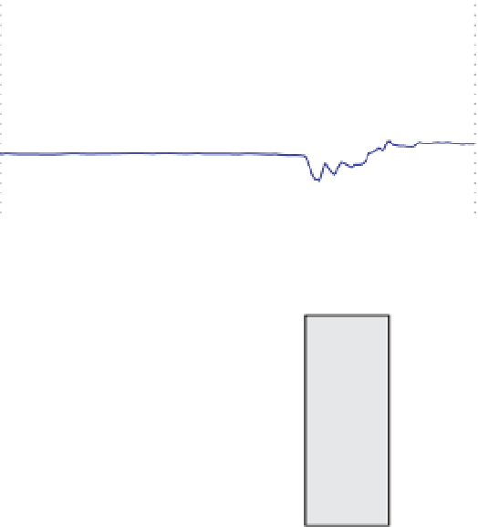
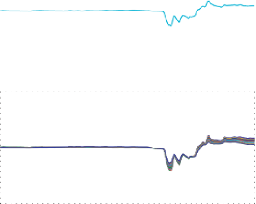
Figure 5.45
Self-potential time series from the water injection experiment.
a)
Raw electrograms.
b)
Detrended and background
corrected electrograms.
c)
Magnification of the electrograms showing the preinjection and injection time windows.
(
See insert for color representation of the figure
.)
direction. We applied the classical inversion algorithm
described earlier to a temporal snapshot of self-potential
data. The kernel was computed using the resistivity
distribution prior to the injection of the water pulse.
The result of the inversion is shown in Figure 5.46a
at the third iteration. The tomogram shows a positive
distribution of the volumetric current density,
defined in Section 5.3), located close to the end of the
open well where the pulse water injection takes place
(Figure 5.46a). This source current density reproduces
the data reasonably well, as shown in Figure 5.46b.
Therefore, we have shown that we successfully deter-
mined the location of the pulse injection of water into
the ground.
(as