Geoscience Reference
In-Depth Information
Y
-position (m)
Thresholded dipole position for top array
0.06 0.07 0.08 0.09 0.10 0.11 0.12
0.12
E3 Time 1851 s
-0.08
E3 Time 1851 s
0.11
Vertical progression
notional section
-0.09
0.10
-0.10
Well
0.09
-0.11
0.08
-0.12
0.07
Void
Well
-0.13
Epoxy
0.06
0.20 0.21 0.22 0.23 0.24
0.25
0.26
E3
Water
X
-position (m)
(a)
(b)
Y
-position (m)
Thresholded dipole position for top array
0.06 0.07 0.08 0.09 0.10 0.11 0.12
0.12
-0.08
E2 Time 1809.5 s
E2 Time 1809.5 s
0.11
-0.09
0.10
-0.10
Well
0.09
-0.11
0.08
E2
-0.12
0.07
Well
-0.13
0.06
0.20 0.21 0.22 0.23 0.24
0.25
0.26
X
-position (m)
(c)
(d)
(e)
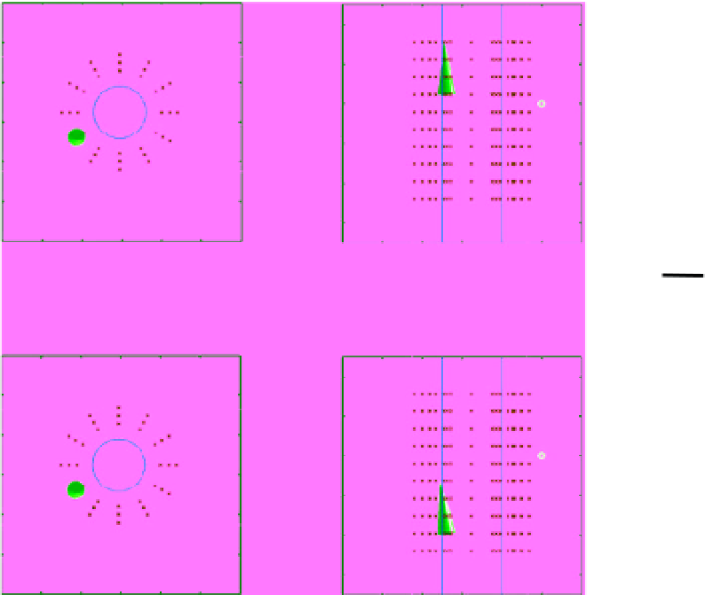
Figure 5.34
Proposed explanation of the electrical disturbances observed in the experiment. Events E2 and E3 are shown together
with their spatial placement near Hole 9 in panels
a)
through
d)
. The blue
x
s in panels
a)
through
d)
are the dipole point
positions used in the genetic algorithm source inversion process. The green circle in panels
a)
and
c)
represents the position of
Hole 9 as viewed from the top, and the vertical green lines in panels
b)
and
d)
represent the position of Hole 9 as seen from the
side. The red circles in panels
b)
and
d)
are the position of one of the measurement electrodes. It can be clearly seen in this
figure that the first event, E2, occurs lower in the model representation (and by correlation, in the test specimen) than the later
event, E3. The figure in panel
e
represents a conceptualization of the movement of the fluid through multiple epoxy barriers,
filling voids in between each the barriers with water. The voids represent points of open contact with the cement that allow
the fracturing fluid to make direct contact, generating the observed pressure fluctuations and electrical impulses.
e)
Sketch of the
tubing showing the progression of the Events E2 and E3 along the well over time.
(
See insert for color representation of the figure
.)
'
E2 being lower in the block than the later in time Event
E3. This clearly shows the upward fluid movement that
was found through the inversion of the data, and
matches with the physical observation of leakage of fluid
at the top of the block, later in the experiment.
data sets, and the results show a very good SNR for both
of these data sets. The base SNR for the pressure data
was computed during the constant pressure phase of the
experiment, before the pressure increases in the constant
flow phase of the experiment. This portion of the signal
had a mean pressure of 1169.8 kPa with an RMS noise
contribution of 1.4 kPa. This noise is what is used to
compute the SNR of the pressure fluctuations that caused
the leakage that was detected electrically. The smallest
5.3.6.3 Noise and position uncertainty analysis
To see how robust the inversion solutions are, a noise
analysis was performed on the voltage and the pressure