Geoscience Reference
In-Depth Information
0
0.1
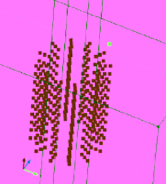
Figure 5.27
COMSOL geometry used
for the fine geometry kernel matrix
computations (360 positions).
a)
Finer
resolution cylindrical kernel matrix
point distribution along with the
measurement points used with the
genetic algorithm.
b)
Close-up of the
kernel matrix point distribution.
(
See insert for color representation of
the figure
.)
0.2
0.3
0.2
0
z
y
0.1
z
0.1
y
0.2
x
0
x
0.3
(a)
(b)
The same analysis was carried out for Event E3
(Figures 5.25 and5.26). The fundamental results for Event
E2 apply to Event E3 with a notable difference. The main
dipole shown in Figure 5.26c is positioned at the same
x
5.3.6.2 Results of the GA
Figure 5.28 shows the results of the GA single dipole
search for Event E2. Figure 5.28a shows a plot of the data
misfit error per Equation (5.45) for each dipole position
(the best solution is highlighted by the small red circle,
Dipole #42). The black line in the figure represents the
minimum of the data misfit error for comparison with
other dipole position optimizations. This figure also
shows how several other dipole positions come close to
the minimum value of the data misfit error. These other
points are at positions 11, 12, and 41. Because of the
COMSOL point sequence, these point positions represent
spatially adjacent or nearly adjacent positions, indicating
that the dipole point matrix may not be positioned in a
manner that places a dipole in the exact position of the
hydromechanical disturbance. It could also indicate that
the disturbance has a volume that encompasses more
than a single dipole point, requiring more than one
dipole point as the solution. Other forms of inversion
and analysis may be able to resolve this uncertainty.
However, for this analysis, the general location of the
centroid of the leak is sufficient to characterize the
problem.
Figure 5.28b shows the comparison of the real data
with the forward model of the dipole that represents
the minimum of the objective function. The synthetic
data reproduces all of the major features of the real data
with an improved L2 norm relative to the coarse gradient
inversion results. The model vector for Dipole #42 is
shown in Figure 5.28c. Note the three positions that have
nonzero values. These values represent the orthogonal
components of the dipole moment found by the GA.
y
location as the dipole responsible for Event E2 in
Figure 5.24c. However, the
z
-axis position of the main
dipole shown in Figure 5.26d has moved up along Hole 9.
This is consistent with the centroid of a hydromechanical
disturbance moving upward along Hole 9 over time.
From the inverted data, it can be seen that the full
model inversion vectors produce excellent matches to
the real data but contain nonphysical elements because
we expect a localized source. The thresholded models
get rid of the nonphysical elements but yields, as
expected, a solution that fits the data with a larger data
RMS error. This increase in RMS error is expected
because the coarse physical positions of the kernel matrix
points used in this inversion do not perfectly match the
true position and geometry of the source current density
of the actual hydromechanical disturbance.
In conclusion, the result of the gradient-based
inversion approach used in phase 1 provides reasonable
estimation for the centroid of current dipole source loca-
tions at different times. We know from AE (not shown
here) and pressure data that there was no fracturing of
the block during the experiment reported in this paper.
Therefore, all dipole solutions located far from Hole 9
are considered not to have a physical cause, given that
the current source is expected to be compact. The coarse
nature of the inversion process calls for refinement;
therefore, this first set of solutions is used to direct the
refinement of the source localization using the GA.
-