Geoscience Reference
In-Depth Information
−100
−150
−200
−250
−300
−350
−400
−450
−500
−550
100 150 200 250 300 350 400 450 500
100 150 200 250 300 350 400 450 500
100 150 200 250 300 350 400 450 500
x
-coordinate (m)
x
-coordinate (m)
x
-coordinate (m)
(a)
(b)
(c)
−100
−150
−200
−250
−300
−350
−400
−450
−500
−550
100 150 200 250 300 350 400 450 500
100 150 200 250 300 350 400 450 500
100 150 200 250 300 350 400 450 500
x
-coordinate (m)
x
-coordinate (m)
x
-coordinate (m)
(d)
(d)
(e)
(e)
(f)
(f)
1
−100
−150
−200
−250
−300
−350
−400
−450
−500
−550
0.9
0.8
0.7
0.6
0.5
0.4
0.3
0.2
0.1
0
100 150 200 250 300 350 400 450 500
100 150 200 250 300 350 400 450 500
x
-coordinate (m)
x
-coordinate (m)
(g)
(h)
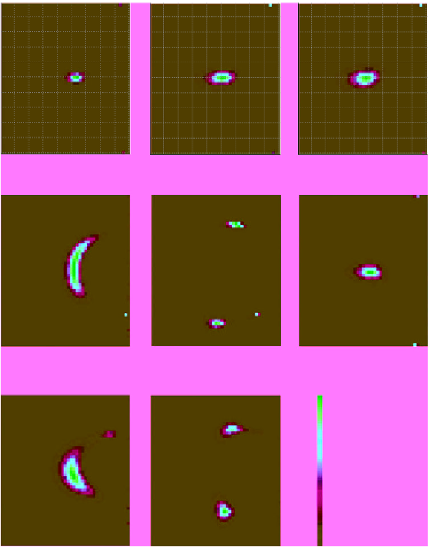
Figure 4.22
Source localization for the electrical potential distributions shown in Figure 4.21 (shot #3). The sources are analyzed
in terms of volumetric source current distributions. The white line indicates the position of the discontinuity between the units
U1 and U2.
a)
Source current distribution at time 184.96 ms.
b)
Source current distribution at time 187.77 ms.
c)
Source
current distribution at time 190.58 ms.
d)
Source current distribution at time 193.38 ms.
e)
Source current distribution
at time 196.19 ms.
f)
Source current distribution at time 210.23 ms. (
See insert for color representation of the figure
.)
a snapshot of the seismoelectric generated source on the
interface, which is shown on a normalized scale in
Figure 4.22. Afterward, the normalized source distribu-
tions at all time steps are aggregated to produce the
tomogram presented in Figure 4.23 that depicts the
presence of a vertical contact at
x
= 300 m. The volumetric
source current distributions are thresholded according to
the global threshold level found by using theOtsumethod