Geoscience Reference
In-Depth Information
Seismic sources
Receivers
Borehole #2
Borehole #2
Borehole #1
Borehole #1
0
100
200
300
400
500
600
0
100
200
300
400
500
600
0
0
PML
PML
R#1
R#1
-100
-100
Unit #1
(U1)
S#1
S#1
-200
-200
Unit #1
(U1)
Unit #2
(U2)
Unit #2
(U2)
-300
-300
-400
-400
S#5
S#5
-500
-500
R#50
R#50
PML
PML
-600
-600
Coordinate
x
(m)
Coordinate
x
(m)
(a)
(b)
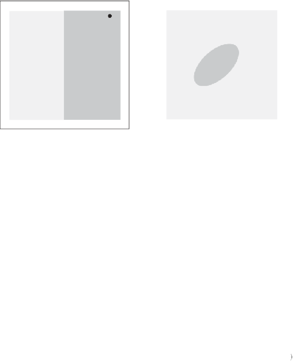
Figure 4.15
The model domain is a 600 m × 600 m square. Borehole #1, the shooting borehole, is located at position
x
= 100 m,
and the measurement borehole #2 is located at
x
= 500 m. The discretization of the domain comprises a finite-element mesh of
60x60 rectangular cells. We consider 5 seismic sources (from S#1 at the top to S#5 at the bottom), equally spaced in borehole #1,
and 50 receivers (R#1 to R#50), located in borehole #2. PML boundary conditions are used at the borders of the domain.
a)
Case
study #1 concerns a vertical interface separating two homogeneous half-spaces. This interface is located at
x
=300 m, an equal
distance between the two sources.
b)
Case study #2 corresponds to an inclusion, U2, embedded into a homogeneous material, U1.
the coseismic signal occurs at
t
2
= 0.313 s. This is in
agreement with the numerical results of Figure 4.18.
Using the relationship between the wavelength and the
velocity of the P-waves,
where (
x
s
,
y
s
,
z
s
) denote the coordinates of the each point
where the seismoelectric conversion takes place. Two
assumptions are made in order to transform the 3D
problem into a 2.5D problem. It is assumed that the model
is homogeneous
λ
S
=
c
p
/
f
, where
f
is the dominant
frequency, the first Fresnel zone radius for the seismic
wave is
r
S
=
dc
p
2
f
1 2
. Using
d
= 200 m (Figure 4.15),
f
= 40 Hz, and
c
p
= 1935.5 m s
−
1
in unit U1, we obtain
r
S
= 69 m. Also, using the relationship between the first
seismic Fresnel zone and the seismoelectric Fresnel zone
(see Section 4.2), we obtain
r
SE
= 98 m, which provides
an idea of the lateral resolution of the seismoelectric
method at this frequency.
in the strike direction
y
,that ,
∂
σ
y
= 0, and the strikedirectionextends to infinity
in both directions. Solving the Poisson equation in the
wave number domain, where
k
y
is the wave number in
the strikedirection, andusing theFourier cosine transform,
x
,
y
,
z
∂
∞
0
ψ
ψ
x
,
z
,
k
y
=
x
,
y
,
z
cos
k
y
y dy
4 64
Equation 4.64, in the wave number domain, takes the
following form:
4.4.2 5D electric forward modeling
The Poisson equation governing the electrostatic poten-
tial distribution corresponds to Equation 4.37. The source
term of this Poisson equation is described as a Dirac
(delta) function and a point current source,
I
(in A):
σ
x
,
z
k
y
ψ
−∇
σ
x
,
z
∇
ψ
x
,
z
,
k
y
+
x
,
z
,
k
y
=
I
δ
x
−
x
s
z
z
s
4 65
−
Therefore, the initial Poisson equation is transformed
to a Helmholtz-type differential equation in the wave
r
,
t
=
∇
j
s
=
I
δ
x
−
x
s
δ
y
−
y
s
δ
z
−
z
s
,
4 63