Geoscience Reference
In-Depth Information
8
CS
6
4
IR4
RCS3
IR5
IR1
IR2 IR3
RCS2
RCS1
2
0
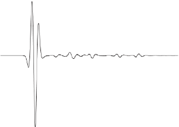
Figure 4.12
Electrogram at an electrode
(receiver) with a horizontal offset of
150 m. CS stands for the coseismic
disturbance associated with the direct
wave (see Figure 4.11). RCS1 and RCS2
stand for the coseismic disturbances
associated with the reflected P-waves
(see Figure 4.11). IRi stand for the
various seismoelectric disturbances
associated with the seismoelectric
conversions at the different interfaces
of the system.
-2
-4
-6
-8
-10
0.1
0.2
0.3
0.4
0.5
0.6
Time (s)
coupling coefficient at the position of the electrode and
the polarity of the seismic waves.
Figure 4.12 shows the electric potential for a given
electrode. In this figure, we can clearly discriminate the
coseismic signals from the seismoelectric conversions.
Note also that the amplitudes of the signals are small.
However, they can easily be measured in the field using
the type of ultrasensitive equipment discussed by Crespy
et al. (2008). This equipment can be used to record the
electrical potential with up to 256 simultaneous channels
at several kHzwitha sensitivityof 10 nV(seeSection4.3.3).
relationships between the porosity, the electrical conduc-
tivity, and the bulkmodulus of the skeleton (Figure 4.13).
4.4 Deterministic inverse modeling
4.4.1 A statement of the problem
The forward computation of the seismoelectric problem is
performed with the finite-element package COMSOL
Multiphysics 3.5a using the same partial differential
equations as Jardani et al
.
(2010). The problem is defined
in COMSOL through the following steps: (1) formulate
the semicoupled field equations that describe the dynamic
poroelastic phenomena with the associated electro-
magnetic disturbances (see Section 4.4.2), (2) define the
geometry of the model (see Figure 4.15), (3) specify the
model parameters (see Table 4.1), (4) design the finite-
element mesh (we use triangular meshing in the present
case), (5) select the boundary layer conditions (we use
PML boundary conditions for the seismic part of the
problem; see Figure 4.15), (6) solve the partial differential
field equations, (7) run the inverse algorithms using the
quasielectrostatic condition, and finally (8) postprocess
the data to produce an image using a pixel-based
approach. The flowchart for this process is shown in
Figure 4.16. The PML boundary conditions consist of a
strip simulating the propagation of the seismic waves
out to infinity without any reflections going back inside
4.3.3 Result of the joint inversion
We use the AMA described in Section 4.4.3 to generate
25,000 realizations of the 21 parameters of the material
properties of the different geological units using the data
recorded in 60 geophones and 60 electrodes at only four
frequencies (25, 30, 35, and 40 Hz). The position and the
characteristic of the source are assumed to be perfectly
known. The posterior probability distribution functions
of the material properties of the three units (layers L1
and L2 and the reservoir R) are shown in Figure 4.13
using the last 5000 iterations. We observe that, except
for the porosity, our algorithm does a very good job of
properly inverting the seismic and seismoelectric data
in terms of finding themean value of thematerial proper-
ties. We believe that a better estimate of the porosity can
be obtained through the use of additional petrophysical