Geoscience Reference
In-Depth Information
Well A (injector)
Well B (producer)
Water
Oil
PML
Distance (m)
-30
0
250
280
30
E1
PML
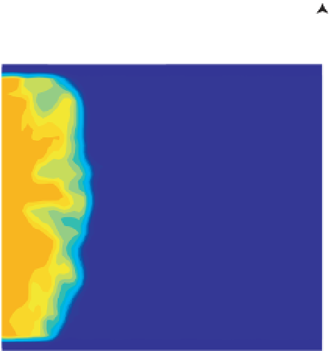
Figure 4.5
Sketch of the domain used
for the modeling. The total modeling
domain is a 410 m× 250 m rectangle.
Injector Well A is used, located at
position
x
=0 m, and is also used for the
seismic source. Production and recording
Well B is located at
x
=250 m. The
discretization of the domain comprises
a finite-element mesh of 205 × 125
rectangular cells. 28 receivers are located
in Well B, approximately 30 m away
from the nearest PML boundary
(the PML boundary layers are shown
in gray). (
See insert for color representation
of the figure
.)
Reservoir
So
E16
PML
E28
180
PML
Seismic source
Receivers
regions simulating therefore propagation to infinity (see
previous equations for damping).
Step 2. We compute the electrical problem using
the electrical conductivity equation developed in
Chapter 1 with
m
=
n
= 2 and a surface conductivity
σ
seismoelectric (SE) conversions occur in each snapshot.
These conversions always arrive earlier than the coseismic
electrical field associated with the arrival of the P-wave.
They also arrive later and later as the water front
progresses toward Well B. This shows that there is a clear
conversionmechanismat theNAPL/water encroachment
front for each of the five snapshots, T2
S
=001 S m
−
1
while the conductivity of the pore water
is 0.1 S m
−
1
. The charge density
Q
0
V
is determined from
the distribution of the permeability (see Chapter 1).
The source current density is determined from the Darcy
velocity and the displacement of the solid phase. Finally,
the electrical potential distribution is obtained by solving
a Poisson equation for the electrical potential.
T6. For snapshot
T1, since there is no saturation contrast, we do not see
any strong seismoelectric conversions. That said, there
are still some small seismoelectric conversions taking
place at the heterogeneities in the aquifer.
Putting the saturation profile T4 into the model, we
show that both the seismoelectric conversion (SE)
generated at the NAPL/water encroachment front and
the coseismic (CS) electrical signals are shown at all
receiving stations E1 to E28 (Figure 4.5 for the position
of the electrodes). Figure 4.7 shows the seismic displace-
ment and the electrical time series for station E12
with information on the delay time
t
0
, seismoelectric
conversion at time
t
1
, and the similarities of coseismic
and P-wave arrival times
t
2
.
In terms of amplitudes, the type of signal measured
here is easily recordable in the laboratory and in the field
through stacking. Dupuis, Butler, and colleagues have
developed methods to improve the signal-to-noise ratio
-
4.2.3 Results
The evolution of the seismic displacement and the
electrical potential time series recorded at station E12
(see Figure 4.5) for each saturation profile (T1
T6) are
shown in Figures 4.6. The seismic displacements are
generated fromthe seismic sourcewhich is a P-wave-only
source. In this case, with the porosity distribution
displayed in Figure 4.3 and with the water saturation
variations shown in Figure 4.4, the average P-wave
velocity of profiles, T1
-
T6, is about 4800 m s
−
1
. The
P-wave arrivals in Well B are therefore roughly the same
in the snapshots T1
-
-
T6 (Figure 4.6). Figure 4.6 shows that