Biology Reference
In-Depth Information
Both RW and PSE simulations of this benchmark case are performed
with varying numbers of particles in order to study spatial convergence.
49
The boundary condition at
x
=
0 is satisfied using the method of images
as introduced in Sec. 7.2.2.
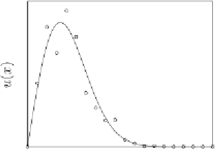
Figure 8 shows the RW and PSE solutions in comparison to the exact
solution at a final time of
T
=
10 for
N
=
50 particles and a diffusion con-
stant of
D
10
−4
. The accuracy of the simulations for different numbers
of particles is assessed by computing the final
L
2
error
=
12
È
˘
N
1
Â
((,
2
L
=
Í
Í
uxT uxT
) (,
-
)
˙
˙
(34)
2
ex
p
p
N
Î
˚
p
=
1
for each
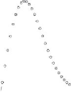
N
. The resulting convergence curves are shown in
Fig.
9. For
RW, we observe the characteristic slow convergence of
O
(1/
√
N
).
68
For
PSE, a convergence of
(1/
N
2
) is observed, in agreement with the
employed second-order kernel function. Below an error of 10
−6
, machine
precision is reached. It can be seen that the error of a PSE simulation
O
0.5
0.5
0.4
0.4
0.3
0.3
0.2
0.2
0.1
0.1
0
0
0
1
2
3
4
0
1
2
3
4
x
x
Fig. 8.
Comparison of (a) RW and (b) PSE solutions of the benchmark case. The
solutions at time
T
10 are shown (circles) along with the exact analytic solution
[solid line; Eq. (33)]. For both methods,
N
=
=
50 particles, a time step of
δ
t
=
0.1,
and
D
=
10
−4
are used. The RW solution is sampled in 20 intervals of width
δ
x
=
0.2.
For the PSE, a core size of
=
h
is used.