Agriculture Reference
In-Depth Information
q(d)
q
q
′
θ
θ
′
d
′
delivery date
d
d
d
L
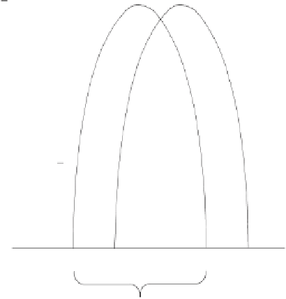
Figure 8.2
Timeliness costs with asset contracting
Figure 8.2 shows the simple case in which the stage length does not differ from its
expectation (
L
=
L
d
0
> d
0
. The optimal time might also change because
) but begins later, at
of changes in the stage length (
L
), changes in the relationship between output and time
(
), or various combinations of these and changes in the time at which the stage
begins. We also ignore the possibility that use of the asset takes place over several days
rather than a single day. The ex post optimal delivery time is now
q
=
q(d)
d
> d
, which would still
d
q
generate the optimal output
. However, because the contract specifies delivery at
, the
q
< q
output will be reduced to
. Depending on how sensitive this particular stage is to the
timing of asset use, output could be drastically reduced or hardly affected. Figure 8.2 shows
a reduction in output by roughly 25 percent from optimal. In the worst case, the entire stage
could shift so far that the output, for the contracted time (
d
), could be zero. The size of these
timeliness costs varies dramatically across crops and across stages for a given crop. Some
implications of this variance are examined in our empirical analysis.
With the addition of timeliness costs to the model, first-best input levels require not only
specialization and perfect incentives but also optimal timing in their application. Short-
term contracting will make such timing quite costly. We assume that timeliness costs do