Biomedical Engineering Reference
In-Depth Information
(b)
(a)
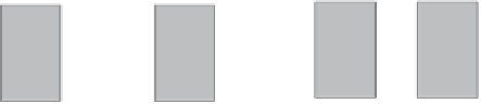
Fig. 6.5.
Two snapshots of the labial motion in the two-mass model. In this model
it is assumed that, if the labia form a convergent profile (the lower parts of the
opposing labia are more separated than the upper parts) as shown in (
a
), the
pressure between the upper parts of the opposing labia is basically the vocal-tract
pressure. On the other hand, the pressure between the lower parts of the opposing
labia is a fraction of the bronchial pressure. If the labia form a divergent profile
as in (
b
), it is considered that the air acquires a velocity in its passage through
the space between the lower parts of the labia such that a laminar regime cannot
be established in the region between the upper parts. On the contrary, a jet is
established, so that the actual value of the distance between the upper parts of the
labia is irrelevant
of the labia is irrelevant. The interface of interest is now the one between
the trachea and the lower part of the labia. For reasons of continuity, the
interlabial pressure can be assumed to be equal to the tracheal pressure.
These hypotheses are illustrated in Fig. 6.5.
The global result of this set of hypotheses is not much different from
that in the case of the flapping model: in both models, the computation of
the average pressure between the labia for a divergent configuration gives
a smaller value than that for a convergent one, thus allowing a net energy
transfer from the airflow to the labial oscillation. The advantage is that if we
use a model in which the upper and lower parts of the labia are elastically
connected instead of having perfectly correlated positions, richer motions are
possible.
The results obtained by studying this model are surprisingly good if we
consider the number of approximations that have been made. Why can we
say that the results are reasonable? First, the equations are stated in such a
way that, given the values of the pressure, the masses that approximate the
labia, the restitution constants of the assumed coupling springs, etc., we are
able to compute the motion of the masses. The equations are simply Newton's
laws applied to this problem:
M
1
x
1
+
B x
1
+
K
1
x
1
+
K
r
(
x
1
−
x
2
)
−
G
1
=
F
1
,
(6.12)
M
2
x
2
+
B x
2
+
K
2
x
2
+
K
r
(
x
2
−
x
1
)
−
G
2
=
F
2
,
(6.13)
where
x
1
,
2
are the departures from equilibrium of the lower and upper masses
M
1
,
2
, respectively;
K
1
,
2
are the restitution constants for each mass;
K
r