Image Processing Reference
In-Depth Information
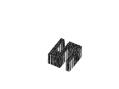
(a)
(b)
FIGURE 1.18: Thinned pattern obtained by ESPTA (a) original 3-D object,
and (b) thinned pattern.
1.4.2 Adjacency Tree
Let C = {C
0
,C
1
,...C
k
} be the set of k disjoint connected components
of foreground and background of a 2-D digital picture P = (G
2
,m,n,S). It
may be noted that foreground components are m-connected and the back-
ground components are n-connected. We further denote F ⊂ C as the set
of foreground components and B ⊂ C as the set of background components.
Two components C
i
and C
j
form an edge, if there exist p ∈ C
i
and q ∈ C
j
such that they are adjacent. In this case, if C
i
is a foreground component,
C
j
must be a background component, and the reverse is also true. Using this
adjacency information, the picture is described in the form of a graph [36],
where vertices are mapped to the foreground and background components,
and edges between two vertices are formed if they are adjacent. It is shown in
[36], that the graph is connected and acyclic, thus forming a tree. This tree is
called an adjacency tree. Let us consider an example of how an adjacency tree
could be formed given a 2-D picture. In Fig. 1.15 a set of foreground object
points (black in color) is shown. If the grid is taken of type (8,4) connectivity,
its set of connected components for foreground and background is shown in
Fig. 1.19(a). In this case, C
1
and C
2
are the foreground components, and B
1
and B
2
are background components. The respective adjacency tree formed by
nodes corresponding to components and edges between two adjacent compo-
nents is shown in Fig. 1.19(b). However, if the pattern of Fig. 1.15 is taken in
a (4,8) grid, the set of connected components and their adjacency tree differ
significantly (see Fig. 1.20). From these figures, we may observe the follow-
ing for an adjacency tree, which is also in general true. These properties are
discussed in [36].
1. The background component containing the border of the picture forms