Cultural Heritage Applications: Archaeological Ceramics and Building Restoration - On Statistical Pattern Recognition in Independent Component Analysis Mixture Modelling - page 130

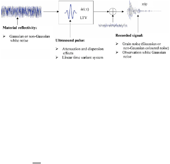
Fig. 6.1 The through-transmission linear time variant model

R

f 2

ð f f c ð t ÞÞ 2 P x ð f ; t Þ df

f 1

Bandwidth BW ð Þ : us ð t Þ¼ BW ð t Þ¼ ð 6 : 3 Þ

R

f 2

P x ð f ; t Þ df

f 1

Maximum frequency amplitude (Afmax): us ð t Þ¼ max P x ð f ; t Þ ð 6 : 4 Þ

These signatures are measures of the spectral content variations that are affected
by the ultrasonic pulse travelling inside the material. They can be estimated by
means of well-known smoothing techniques of time-frequency spectral analysis
[ 7 ].
From us ð t Þ , we can obtain features in different forms. For example, the time

t 1 t 0 R

t 1

1

average value us ð t Þ dt or the instantaneous value at one particular time

t 0

instantus ð t 0 Þ can be elements of the feature vector in the observation space. Other
time-domain features, such as the parameters A and b corresponding to an expo-
nential model of the signal attenuation x ð t Þ¼ Ae bt or the total signal power

received P ¼ R 0

j x ð t Þj 2 dt =: T ; are also possible to complement the frequency-

domain features.
More features can be defined considering special conditions of the through-
transmission model. For example, higher-order statistics can be used to detect the
possible degree of non-gaussianity of the reflectivity by measuring higher-order
moments of the received signal like HOM ¼ Ex ð nT s Þ x ðð n 1 Þ T s Þ½ x ðð n 2 Þ T s Þ
0, where E ½ means statistical expectation and 1 = T s is the sampling frequency.
Departures from the linear model of Fig. 6.1 can be tested in different forms, for
example, using the so-called time-reversibility [ 8 ], which is defined by

" #

3

dx ð t Þ
dt

TR ¼ E

.