Second-Order Transport Modeling - Transport and Fate of Chemicals in Soils: Principles and Applications - page 169

Ω = 0.1

1.0

0.8 1

0.6

5

0.4

10

0.2

0 01234

5678 9 0

V/V o

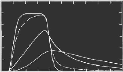
FIGURE 6.8
Effluent concentration distributions for different values of the parameter Ω of the second-order
model. (From H. M. Selim and M. C. Amacher. 1997. Reactivity and Transport of Heavy Metals in
Soils . Boca Raton, FL: CRC Press. With permission.)

such as those defined by Equations 6.17 to 6.22. The use of dimensionless
parameters offers a distinct advantage over the use of conventional param-
eters since they provide a wide range of application as well as further insight
on predictive behavior of the model. Figures 6.8 to 6.10 are simulations that
illustrate the transport of a reactive solute with the second-order model for
selected dimensionless parameters. Unless otherwise indicated the values
for the dimensionless parameters Ω, κ 1 , κ 2 , κ 3 , κ 4 , F , κ s , P , and T p were 5, 1, 1,
0.1, 0.1, 0, 0.5, 25, and 1, respectively.
Figure 6.8 shows BTCs of a reactive solute for several values of Ω. The fig-
ure indicates that the shape of the BTCs is influenced drastically by the value

κ 1 κ 2 κ 3 κ 4

1.0 0.1

1 20

0.1
1 20

0.01
0.1
2

0.01
0.1
2

0.8

0.6 A

B

0.4

D

0.2 C

0 01234

5678 9 0

V/V o

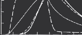
FIGURE 6.9
Effluent concentration distributions for different values of rate coefficients (κ 1 , κ 2 , κ 3 , and κ 4 )
using the second-order model. (From H. M. Selim and M. C. Amacher. 1997. Reactivity and
Transport of Heavy Metals in Soils . Boca Raton, FL: CRC Press. With permission.)