Transport - Transport and Fate of Chemicals in Soils: Principles and Applications - page 94

3.75 is an implicit equation for C and where iteration is necessary. Specifically, a
solution for C at each time step j and iteration step r can be obtained as follows:

H

r + 1

[ ] =

C

(3.76)

ij , + 1

( )

b − 1

r

Θ+ρ [ C ]

K f ij , + 1

All other finite-difference expressions are similar to those described above.

3.9.3 Simulations

In order to illustrate the kinetic behavior of reactive solutes having various
retention mechanisms, the transport model was used to provide a number of
simulations. Figures 3.14 through 3.20 are selected simulations that illustrate
the sensitivity of solution concentration results to a wide range of parameters
associated with equilibrium as well as kinetic retention reactions. The soil
parameters selected for these illustrations are: ρ = 1.25 g cm -3 , Θ = 0.4 cm 3 , L =
10 cm, C i = 0, C o = 10 mg L -1 , and D = 1.0 cm 2 h -1 . Here it was assumed that
a solute pulse was applied to a fully water-saturated soil column initially
devoid of solute. In addition, a steady water-flow velocity ( q ) is assumed con-
stant, with a Peclet number P (= qL /Θ D ) of 25. The length of the pulse was
assumed to be three pore volumes, which was then followed by several pore
volumes of a solute-free solution.
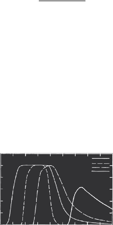
The influence of the Freundlich distribution coefficient K f of the nonlinear
equilibrium type reaction on the transport of dissolved chemicals is shown
in Figure 3.15. The shape of the BTCs reflects the influence of nonlinear

Nonreactive

K f = 1 cm 3 g -1
2
5

1.0

0.8

0.6

0.4

0.2

0 0

1 2 3 4 5 6 7 8 9

V/V o

FIGURE 3.15
Breakthrough curves for several Freundlich K f values and b = 0.5. (From Selim and Amacher,
1997. With permission.)