Agriculture Reference
In-Depth Information
1.0
Tritium
Sharkey soil
0.8
0.6
0.4
0.2
0.0
0
1
2
3
4
5
Pore Volume (V/V
o
)
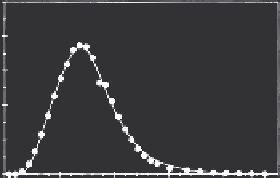
FIGURE 3.13
Tritium breakthrough results (
C
/
C
o
versus
V
/
V
o
) for a Sharkey clay soil. The solid curve is the
fitted breakthrough curve. (From Selim and Amacher, 1997. With permission.)
are not available. Commonly used numerical methods are the finite-differ-
ence explicit-implicit methods (Remson et al., 1971; Pinder and Gray, 1977).
Finite-difference solutions provide distributions of solution (
C
) and sorbed
phase concentrations (
S
e
,
S
1
,
S
2
, and
S
3
) at incremental distances Δ
x
and
time steps Δ
t
as desired. In a finite-difference form a variable such as
C
is
expressed as
C
(
z
,
t
)
=
C
(
i
Δ
z
,
j
Δ
t
),
i
=
1,2,3,…,
N
,
and
j
=
1,2,3,
...
(3.57)
where
z
=
i
Δ
z
,
and
t
=
j
Δ
t
(3.58)
For simplicity the concentration
C
(
x
,
t
) may be abbreviated as:
C(z, t) = C
i, j
(3.59)
where the subscript
i
denotes incremental distance in the soil and
j
denotes
the time step. We will assume that the concentration distribution at all incre-
mental distances (Δ
x
) is known for time
j
. We now seek to obtain a numeri-
cal approximation of the concentration distribution at time
j
+ 1. The CDE
(Equation 3.24) must be expressed in a finite-difference form. For the disper-
sion and convection terms, the finite-difference forms are
−
2
2(
+
2
C
z
C
C
C
+
∂
∂
i
++
1,
j
1
ij
,
+
1
i
−
1 ,
j
+
1
Θ
D
=Θ
D
2
2
z
)
(3.60)
−
2
2(
+
+
C
C
C
i
+
1,
j
ij
,
i
−
1 ,
j
2
×Θ
D
Oz
(
)
2
z
)


Search WWH ::

Custom Search