Aberration Detection in R Illustrated by Danish Mortality Monitoring - Biosurveillance: Methods and Case Studies - page 224

The Farrington algorithm contains a number of additional refinements for
improving the prediction of y t 0 , for example, by correcting for past outbreaks
among the reference values, by testing the need of the trend component in
Equation 12.2, and by a skewness correction of the predictive distribution for
low count series. In order to keep the current presentation compact, we refer
to Farrington et al. (1996) for further details on these refinements. In sur-
veillance , the function farrington is used to run the algorithm:

R> phase2 <- which(epoch(momo) >= "2007-10-01")
R> s.far <- farrington (momo[, "[0,1)"], control = list(range
= phase2, alpha = 0.01, b = 5, w = 4, powertrans = "none"))

We start the monitoring in week 40 of 2007 (that is, October 1, 2007) and
let phase2 denote the index of all ISO weeks to monitor. The call to func-
tion farrington then performs aberration detection for these weeks in the
<1 age group. Note that all aberration detection algorithms in surveil-
lance follow the same structure: The first argument denotes an object of
class sts containing the data, the second argument contains a list of algo-
rithm-specific control options, and a vector range with the time points to
monitor. Specifically, the above code uses α = 0.01 to form the upper limit
of the predictive distribution, and b = 5 and w = 4 to generate the reference
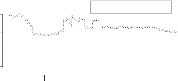
values. Figure 12.3 shows the results of the monitoring. In order to obtain the
above-described procedure without any additional transformation, the argu-
ment powertrans ="none" is used. Other options are "2/3", which provides
a skewness correction, which is preferable in low count scenario. Similarly,
"1/2" provides the variance stabilizing square-root transformation.

None 1/2 2/3

30

20

^

10 µ t 0

0

2007 2008 2008 2008

IV II III IV

Time (weeks)

Figure 12.3
Aberration detection for the <1 age group using the Farrington et al. (1996) method. The upper
three lines show the upper prediction limit as calculated using each of the three possible power
transformations. The lower solid line denotes the expected model predicted number of cases
for each time point t 0 . Triangles indicate an alarm.