Biology Reference
In-Depth Information
25
1500
20
15
1000
10
500
5
0
0
1994
1997
2001
2004
2008
1994
1997
2001
2004
2008
II
IV
II
IV
II
II
IV
II
IV
II
Time (weeks)
Time (weeks)
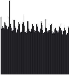
Figure 12.2
(Left) Weekly number of all-cause deaths in Denmark 1994-2008 aggregated over all age
groups, and (right) the weekly data of the <1 age group. The increase of mortality in this group
is due to a change in the gestational age defining a stillbirth, which was lowered from 28 weeks
to 22 weeks in 2004.
R> plot(momo[year(momo) >= 2000, ], type = observed time |
unit)
R> plot(momo, ylab = "No. of deaths", type = observed time)
R> plot(momo[, "[0,1)"], ylab = "No. of deaths")
In the above lines, the type argument controls the view on the multivari-
ate time series object. If no such argument is provided as in the third call, a
default choice is used.
Figure 12.1 shows that monitoring of weekly mortality in Denmark
requires handling both weekly time series containing small count num-
bers and series having large counts. For the four age groups in the top row
of the figure, it will be important to take the count data nature into account,
because a Gaussian approximation is expected to work poorly here. As a
consequence, we will in our work focus on statistical modeling and aber-
ration detection handling small counts. The methods should, however, be
flexible enough to also handle time series with large counts as, for example,
in the bottom row of Figure 12.1. An additional advantage of being able to
handle small counts is that this also allows for further stratification of the
data into, for example, geographical regions or gender. Furthermore, the
time series can contain temporal trends, such as the downward trend for
the 65-74 group or the mortality increase in the ≥85 group due to increas-
ing longevity. Similar examples are the seasonal patterns for the 75-84 and
≥85 age groups, where an increased mortality during winter and spring
is observed. In order to accommodate such nonstationarity, we want to


