Information Technology Reference
In-Depth Information
1.1
g
=
0.1
1.08
G
1.06
1.04
1.02
1
0
−
3
−
2
0.2
−
1
0.4
0
0.6
1
k
h
g
=
0.05
0.8
2
3
1
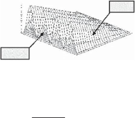
Figure 2.2
Weight modulus increment surfaces for
g
= 0
.
1(exterior)and
g
= 0
.
05 (interior).
k
is expressed in radians.
for low learning rates (as near convergence), the increase of the weight modulus
is less significant. Consider now the ratio
G
,definedas
2
2
G
=
w (
t
+
1
)
+
gh
sin
2
2
=
1
ϑ
x
w
2
2
w (
t
)
=
G
(
g
(α (
t
)
,
w (
t
)
2
)
,
h
,
ϑ
x
w
)
(2.99)
4
2
and
where
h
=
x
(
t
)
2
+
α
(
t
)
4
!
4
2
w (
t
)
for LUO
2
+
α
(
t
)
4
g
=
(2.100)
w (
t
)
2
for OJAn
"
2
+
α
(
t
)
4
)
−
4
2
w (
t
for EXIN
Figure 2.2 represents the portion of
G
greater than 1 (i.e., the modulus increment)
as a function of
h
(here normalized) and
ϑ
x
w
=
k
∈
(
−
π
,
π
], parameterized by
g
. It shows that the increment is proportional to
g
.
The following considerations can be deduced:
• Except for particular conditions,
the weight modulus always increases
:
2
2
2
2
w (
t
+
1
)
>
w (
t
)
(2.101)
These particular conditions (i.e., all data in exact particular directions) are
too rare to be found in a noisy environment.
• The weight modulus does not increase (
G
=
1) if the parameter
g
is null.
In practice, this happens
only
for
α (
t
)
=
0.
• The parameter
g
gives the size of the weight modulus increment. If
g
→
0,
then
G
→
1. Equation (2.100) shows that
g
is related to the weight modulus
according to a power depending on the kind of neuron. MCA EXIN has the
biggest increment for weight moduli less than 1; this explains the fact that it


Search WWH ::

Custom Search