TOTAL LEAST SQUARES PROBLEMS - Neural-based Orthogonal Data Fitting: The EXIN Neural Networks - page 8

x 1

x ′ 1

r 1

x ′

⊥ R 1 ([A;b ′ ])

− 1

r 2

− 1

x 3

R([A;b ])

′

x ′ 2

r 3

x 2

(a)

∧

x 1

x 1

r 1

∧

∧∧

x

⊥ R([A;b ′ ])

− 1

r 2

− 1

x 3

∧ ∧

R([A;b])

x 2

r 3

x 2

(b)

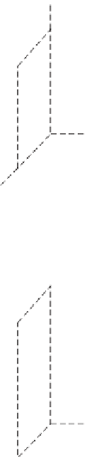
Figure 1.1 Geometry of the LS solution x (a) and of the TLS solution x (b) for n = 2. Part
(b) shows the TLS hyperplane.

Definition 15 The TLS hyperplane is the hyperplane x n + 1 =− 1 .

The LS approach [for n = 2, see Figure 1.1(a)] looks for the best approximation
b to b satisfying (1.5) such that the space R r ( [ A ; b ] ) generated by the LS
approximation is a hyperplane. Only the last components of r 1 , r 2 , ... , r m can
vary. This approach assumes random errors along one coordinate axis only. The
TLS approach [for n =

b ] )
such that (1.9) will be satisfied. The data changes are not restricted to being
along one coordinate axis x n + 1 . All correction vectors

2, see Figure 1.1(b)] looks for a hyperplane R r ( [ A ;

r i given by the rows of