Database Reference
In-Depth Information
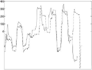
Fig. 9.
Left:
Two sequences and their mean values.
Right:
After normalization. Obvi-
ously an even better matching can be found for the two sequences.
The sequences represent data collected through a video tracking process
(see Section 6). The
DTW
fails to distinguish the two classes of words, due
to the great amount of outliers, especially in the beginning and in the end of
the sequences. Using the Euclidean distance we obtain even worse results.
Using the
LCSS
similarity measure we can obtain the most intuitive clus-
tering as shown in the same figure. Even though the ending portion of the
Boston 2
time-series differs significantly from the
Boston 1
sequence, the
LCSS
correctly focuses on the start of the sequence, therefore producing
the correct grouping of the four time-series.
2. Simply normalizing the time-series (by subtracting the average value)
does not guarantee that we will achieve the best match (Figure 9). How-
ever, we are going to show in the following section, that we can try a
set of translations which will provably give us the optimal matching (or
close to optimal, within some user defined error bound).
4. Ecient Algorithms to Compute the Similarity
4.1.
Computing the Similarity Function S
1
To compute the similarity functions
1wehavetoruna
LCSS
compu-
tation for the two sequences. The
LCSS
can be computed by a dynamic
programming algorithm in
S
O
n
∗
m
) time. However we only allow matchings
when the difference in the indices is at most
(
, and this allows the use of a
faster algorithm. The following lemma has been shown in [12].
δ
Lemma 1.
Given two sequences A and B, with
|A|
=
n
and
|B|
=
m
,we
can find the
LCSS
δ,ε
(A,B) in
O
(
δ
(
n
+
m
))
time.