Database Reference
In-Depth Information
Space Shuttle
Sine Cubed
Noisy Sine Cubed
1
1
1
0.8
0.8
0.8
0.6
0.6
0.6
0.4
0.4
0.4
0.2
0.2
0.2
0
0
0
1
2
3
4
5
6
1
2
3
4
5
6
1
2
3
4
5
6
ECG
Manufacturing
Water Level
1
1
1
0.8
0.8
0.8
0.6
0.6
0.6
0.4
0.4
0.4
0.2
0.2
0.2
0
0
0
1
2
3
4
5
6
1
2
3
4
5
6
1
2
3
4
5
6
Tickwise 1
Tickwise 2
Exchange Rate
1
1
1
0.8
0.8
0.8
0.6
0.6
0.6
0.4
0.4
0.4
0.2
0.2
0.2
0
0
0
1
2
3
4
5
6
1
2
3
4
5
6
1
2
3
4
5
6
Radio Waves
1
1
0.8
0.8
0.6
0.6
0.4
0.4
0.2
0.2
1
2
3
4
5
6
0
E*2
E*2
E*2
E*2
E*2
E*2
0
1
2
3
4
5
6
1
2
3
4
5
6
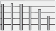
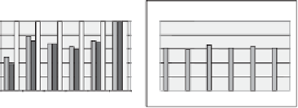
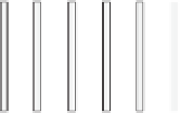
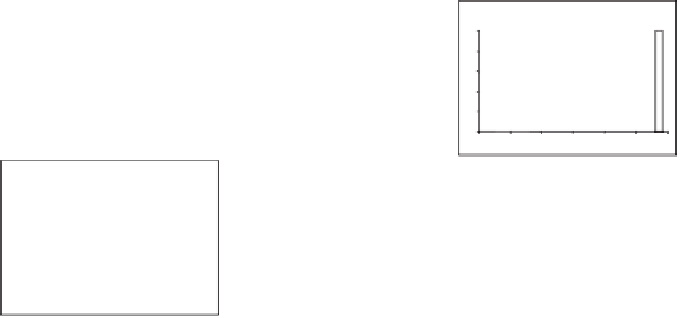
Fig. 5. A comparison of the three major times series segmentation algorithms, on ten
diverse datasets, over a range in parameters. Each experimental result (i.e. a triplet of
histogram bars) is normalized by dividing by the performance of the worst algorithm on
that experiment.
approaches produce better results, but are oine and require the scan-
ning of the entire data set. This is impractical or may even be unfeasible in
a data-mining context, where the data are in the order of terabytes or arrive
in continuous streams. We therefore introduce a novel approach in which
we capture the online nature of Sliding Windows and yet retain the supe-
riority of Bottom-Up. We call our new algorithm SWAB (Sliding Window
and Bottom-up).
4.1.
The SWAB Segmentation Algorithm
The SWAB algorithm keeps a buffer of size
. The buffer size should ini-
tially be chosen so that there is enough data to create about 5 or 6 segments.
w