Database Reference
In-Depth Information
(i)
(vi)
(ii)
(vii)
(iii)
(viii)
(iv)
(ix)
(v)
(x)
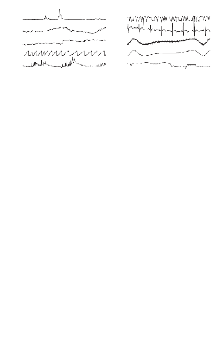
Fig. 3. The 10 datasets used in the experiments. (i) Radio Waves. (ii) Exchange
Rates. (iii) Tickwise II. (iv) Tickwise I. (v) Water Level. (vi) Manufacturing. (vii) ECG.
(viii) Noisy Sine Cubed. (ix) Sine Cube. (x) Space Shuttle.
distance is just the square root of the sum of squares). Euclidean dis-
tance, or some measure derived from it, is by far the most common metric
used in data mining of time series [Agrawal
et al.
(1993), Agrawal
et al.
(1995), Chan and Fu (1999), Das
et al.
(1998), Keogh
et al.
(2000), Keogh
and Pazzani (1999), Keogh and Pazzani (1998), Keogh and Smyth (1997),
Qu
et al.
(1998), Wang and Wang (2000)]. The linear interpolation ver-
sions of the algorithms, by definition, will always have a greater sum of
squares error.
We immediately encounter a problem when attempting to compare the
algorithms. We cannot compare them for a fixed number of segments, since
Sliding Windows does not allow one to specify the number of segments.
Instead we give each of the algorithms a fixed
max error
and measure the
total error of the entire piecewise approximation.
The performance of the algorithms depends on the value of
max error
.
As
max error
goes to zero all the algorithms have the same performance,
since they would produce
/2 segments with no error. At the opposite end,
as
max error
becomes very large, the algorithms once again will all have
the same performance, since they all simply approximate T with a single
best-fit line. Instead, we must test the relative performance for some rea-
sonable value of
max error
, a value that achieves a good trade off between
compression and fidelity. Because this “reasonable value” is subjective and
dependent on the data mining application and the data itself, we did the fol-
lowing. We chose what we considered a “reasonable value” of
max error
for
each dataset, and then we bracketed it with 6 values separated by powers of
two. The lowest of these values tends to produce an over-fragmented approx-
imation, and the highest tends to produce a very coarse approximation. So
in general, the performance in the mid-range of the 6 values should be
considered most important. Figure 4 illustrates this idea.
n