Database Reference
In-Depth Information
G
1
:
G
2
:
G
3
:
1
2
1
2
1
2
1
3
1
3
1
3
3
3
3
1
1
1
4
4
4
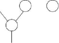
Fig. 3.
Three graphs (
G
1
,G
2
,G
3
).
2
G
1
:
1
3
3
1
4
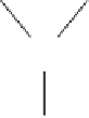
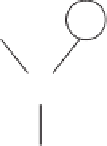
Fig. 4.
The median of (
G
1
,G
2
,G
3
) in Fig. 3 using
d
2
.
We conclude this section with an example of median graph under graph
distance
G
3
are shown in Figure 3.
Their median is unique and is displayed in Figure 4.
d
2
. Three different graphs
G
1
,
G
2
,and
6. Median Graphs and Abnormal Change Detection in
Sequences of Graphs
The measures defined in Sections 3 and 4 can be applied to consecutive
graphs in a time series of graphs (
G
1
,...,G
n
) to detect abnormal change.
That is, values of
d
(
G
i−
1
,G
i
) are computed for
i
=2
,...,n
, and the change
from time
G
i−
1
,G
i
) is larger than a
certain threshold. However, it can be argued that measuring network change
only between consecutive points of time is potentially vulnerable to noise,
i.e., the random appearance or disappearance of some vertices together
with some random fluctuation of the edge weights may lead to a graph
distance larger than the chosen threshold, though these changes are not
really significant.
One expects a more robust change detection procedure is obtained
through the use of median graphs. In statistical signal processing the median
i −
1to
i
is classified abnormal if
d
(