Stability Analysis - Mechanics of Structures: Variational and Computational Methods - page 691

They represent the critical values of the solution path. For a structure, they give the condi-
tions of buckling of either the whole system or of its members. The critical buckling load
follows from the lowest eigenvalue. The corresponding eigenvector or modeshape can be
visualized as the buckling shape or buckling pattern. In addition to the lowest eigenvalue
and corresponding eigenvector, the higher ones may be of interest. This is the case, for
instance, if symmetric and antisymmetric buckling exists.
Another method of determining the buckling load is to assemble separately the linear and
the geometric stiffness matrices and to associate a factor

(a multiplier for the fundamental
state) with the geometric matrix to form the homogeneous system

λ

KV = ( K lin + λ K geo ) V = 0 (11.67)

This possibility is applicable only if the stiffness can be separated into linear and geometric
parts, which is not the case for analytical solutions, because they usually lead to transcen-
dental functions or higher power series.

11.5.2 Determination of the Buckling Loads Using Analytical Solutions

=

For the analytical solutions of Section 11.2.4, the condition det K 0 leads to equations

with transcendental functions with, in general, an infinite number of roots. The determi-
nation of the corresponding eigenvalues and eigenvectors is rather involved [Zurm uhl,
1963], but gives the full spectrum of information. This procedure is applied mostly for
beams and small structures. The following two examples will demonstrate the proce-
dure to set up the problem and find the roots. In addition to the resulting two eigen-
values, which represent the first and second bifurcation (or buckling) loads, the correspond-
ing eigenvectors are given. These buckling shapes portray the buckling behavior of the
structures.

EXAMPLE 11.6 Buckling of a Hinged-Hinged Beam
Use the condition det K 0tofind the first two bifurcation loads for a hinged-hinged

column. See Fig. 11.27a. The lowest bifurcation load is referred to as the Euler load of this
beam column. More specifically, these are four cases of Euler loads corresponding to four
different boundary conditions. The hinged-hinged beam is usually labeled as Euler case 4.
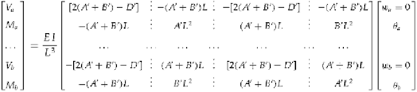
The kinematic boundary conditions

=

0 applied to the stiffness equations
of Eq. (11.50), in which the longitudinal motion terms are ignored, gives

w = 0 and w =

a b

(1)

The first and third rows and columns vanish. Equation (11.66) corresponds to the determi-
nant of the four remaining terms being zero. Then

A 2 B 2

= = ( − ) =

det K 0 EIL 0 (2)