Information Technology Reference
In-Depth Information
Then, sum these parts of the local stiffness matrix of element 1.
k
total
=
k
1
k
lin
+
k
geo
=
(
u
X
1
)
(θ
)
(
u
X
2
)
(θ
)
Y
1
Y
2
V
1
F
X
1
M
1
M
Y
1
V
2
F
X
2
M
2
M
Y
2
1941
.
92
−
8325
.
86
−
1941
.
92
−
8325
.
86
43 809
.
20
8325
.
86
22 797
.
70
=
(3)
Symmetric
1941
.
92
8325
.
86
43 809
.
20
U
1
=
0
=
0
U
2
1
2
The transformation of the local stiffness matrices of element 1 to global coordinates is
accomplished by setting
The displacements and forces in parentheses above and
to the right of the matrix of (3) indicate the local and global variables to assist in identifying
where the rows and columns fit when assembling the nodal equilibrium equations in the
summation process to obtain the system stiffness matrix.
In contrast to the expressions arising from the analytical solution, the loading vector for
the approximation with the geometric stiffness does not contain geometrically nonlinear
terms. From Eq. (4.73)
w
=
U
2
.
2
V
1
1
F
1
X
1
M
1
1
M
1
Y
1
V
1
2
F
1
X
2
M
1
2
M
1
Y
2
36
.
00
−
/
2
−
48
.
00
2
12
−
/
/
p
10
−
=
w
=
(4)
36
.
00
2
48
.
00
2
−
/
12
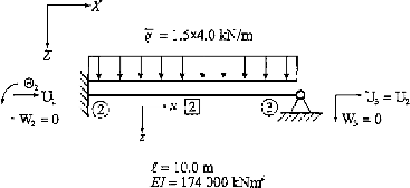
Stiffness Matrix and Load Vector of Element 2
For element 2, a beam, the longitudinal force of the linear fundamental state is zero. This
value is obtained from the linear analysis of the framework as the initial step in the analysis.
Thus, only the elastic part of the stiffness matrix is of importance and is evaluated for the
system fixed at one end with a moment release at the other. This stiffness matrix can be
taken from the fixed-hinged case of Table 11.3. Use the element properties from Fig. 11.23
FIGURE 11.23
Element 2 with local global coordinates.


Search WWH ::

Custom Search