Information Technology Reference
In-Depth Information
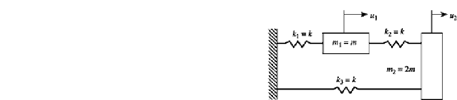
FIGURE 10.5
The two-DOF system for Examples 10.4 and 10.9.
The characteristic equation of the form of Eq. (10.36)
(
|
K
−
λ
M
|=
0
)
is
2
h
−
λ
−
h
=
0
(2)
−
h
2
h
−
2
λ
2
where
h
=
k
/
m,
and
λ
=
ω
.
This reduces to a polynomial
3
2
h
2
2
λ
−
3
h
λ
+
=
0
(3)
√
3
Solve (3) for
λ
, giving
λ
=
(
3
±
)
h
/
2
,
or
1
,
2
796266
k
538188
k
ω
=
0
.
/
m
and
ω
=
1
.
/
m
(4)
1
2
Substitute
ω
2
into Eq. (10.33) to find the mode shapes
φ
1
and
φ
2
. Because
φ
1
and
φ
2
are shapes, i.e., they are relative magnitudes of the DOF obtained from the homogeneous
equations
ω
1
and
2
M
φ
0
,
they can be normalized (scaled) by giving a specific value to
one element in each
φ
and then make the other elements have the same ratio with this
element as before. If the first elements in
φ
1
and
φ
2
are set to 1, then
ω
−
K
φ
=
1
and
φ
2
=
.
000
1
.
000
φ
1
=
(5)
1
.
366025
−
0
.
366025
1
10
m
1
,
it would appear reasonable
to ignore
m
2
. The system becomes a single DOF system with the governing differential
equation
If
m
2
is made very small as compared to
m
1
, say,
m
2
=
3
2
ku
m u
+
=
0
(6)
The natural frequency is
√
1
1
.
5
k
/
m,
w
hereas the exact first natural frequency with
m
2
=
10
m
ω
1
=
√
1
can be calculated as
.
46
k
/
m
.
Then the error of this approximation for the eigenvalue
is
1
.
5
−
1
.
46
=
2
.
74%
(7)
1
.
46
We can improve this approximation by employing Guyan reduction. From Eq. (10.18),
T
=
0
.
5
,
and from Eq. (10.23),
1
2
k
m
=
m
+
0
.
1
×
0
.
25
m
=
1
.
025
m,
k
=
2
k
−
=
1
.
5
k
(8)


Search WWH ::

Custom Search