Information Technology Reference
In-Depth Information
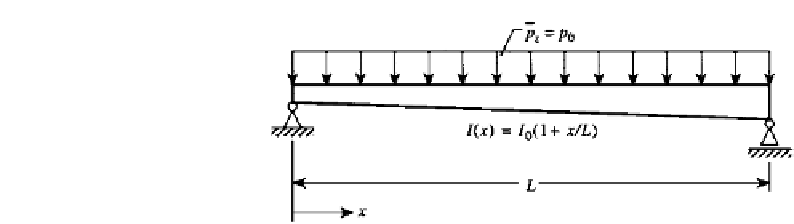
FIGURE 8.4
Beam with a variable cross-section.
EXAMPLE 8.1 Beam of Variable Cross-Section
A simply supported beam will be employed to illustrate the use of finite difference ap-
proximations in the solution of differential equations. Choose the beam of Fig. 8.4 with a
cross-sectional area that varies with a moment of inertia
I
x
L
,
where
I
0
is the
moment of inertia at the left end. We wish to compute the deflection at the quarter points
along this uniformly loaded beam.
Finite difference expressions can be used to integrate the familiar fourth order beam
theory equation or the simpler second order relationship
(
x
)
=
I
0
(
1
+
)
d
2
w
dx
2
=−
EI
(
x
)
M
(1)
We choose to utilize this expression. For the statically determinate beam of Fig. 8.4, the
bending moment is observed to be
p
0
2
p
0
L
2
2
M
=
x
(
L
−
x
)
=
ξ(
1
−
ξ)
(2)
where
ξ
=
x
/
L
.
Of course, this expression satisfies the static boundary conditions
M
(
0
)
=
M
(
L
)
=
0
(3)
Substitute
M
of (2) in (1) to obtain
d
2
p
0
L
2
2
EI
0
p
0
L
2
2
EI
0
w
dx
2
=−
[
(
x
/
L
)(
1
−
x
/
L
)/(
1
+
x
/
L
)
]
=−
[
ξ(
1
−
ξ )/(
1
+
ξ)
]
(4)
The problem is now one of integrating (4) subject to the displacement boundary conditions
w(
0
)
=
w(
L
)
=
0
(5)
It is convenient to normalize
w
using
p
0
L
4
=
w/(
/
2
EI
0
)
(6)
u
so that (4) becomes
d
d
u
=−
ξ(
−
ξ )/(
+
ξ)
=
1
1
(7)
ξ


Search WWH ::

Custom Search