Information Technology Reference
In-Depth Information
For a particular case, retain only those terms corresponding to the actual boundary condi-
tions for the problem. We see that the free parameters
w
can be found from
[
k
u
+
(
R
p
+
R
u
)
]
w
=
p
u
(7.76)
EXAMPLE 7.10 Beam with Linearly Varying Loading
To illustrate the use of a trial function which does not satisfy all boundary conditions, we
return again to the beam of Fig. 7.1. As the first choice of a trial function, use
w
1
w
2
3
4
]
2
N
u
w
=
w
=
[
ξξ
ξ
ξ
(1)
w
3
w
4
This approximate displacement satisfies only the boundary condition
w(
0
)
=
0
,
but not
the conditions
θ(
0
)
=
w(
L
)
=
M
(
L
)
=
0
.
Substitute Eq. (2) of Example 7.9, along with
N
i
u
=
(
L
4
1
/
)
[0 0 0 24]
,
into Eq. (7.75)
ξ
ξ
000 12
000 8
000 6
00024
L
4
1
2
EI
EI
L
4
k
u
=
L
[0
0
0
24]
d
ξ
=
(2)
ξ
3
0
/
5
ξ
4
(
ξ
ξ
1
/
6
p
0
L
1
0
2
/
1
12
p
u
=
1
−
ξ)
d
ξ
=
p
0
L
(3)
ξ
3
/
1
20
ξ
4
1
/
30
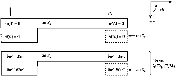
We still need to compute the boundary terms
R
u
and
R
p
.
The formation of these conditions
is illustrated in Fig. 7.6. We find
R
u
=
N
T
)
N
T
u
N
u
(
N
T
u
(
1
)
N
u
(
1
+
)
(
0
)
0
)
−
(
0
)
N
u
(
0
EI
u
(4)
S
u
at
ξ
=
1
S
u
at
ξ
=
0
R
p
=
N
u
(
)
EI
N
u
(
1
)
1
(5)
S
p
at
ξ
=
1
FIGURE 7.6
Boundary displacements and forces for the beam of Fig. 7.1 and corresponding boundary terms for the extended
variational form.


Search WWH ::

Custom Search