Information Technology Reference
In-Depth Information
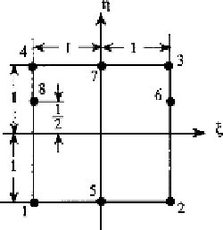
FIGURE P6.20
(
)
6.22 Show that
N
i
of Eq. (6.71) is obtained from the Lagrangian polynomials of Eq.
(6.64) by a transformation from Cartesian to natural coordinates.
6.23 Use one-, two-, and three-point Gaussian quadrature to find values of the following
integrals. Compare your results with the exact solutions.
1.
2
0
L
k
2.
1
−
3.
8
2
1
2
x
4
1
x
dx
x
2
cos
x dx,
1
(
+
)
dx,
=
4
(ξ
+
Hint:
Change of variables: 1.
x
1
)
,3.
x
=
3
ξ
+
5
Answer:
1
.
n
=
1:1
.
1107
n
=
2:0
.
9985
,
n
=
3:1
.
000008
2
.
n
=
1:0
n
=
2:0
.
778
,
n
=
3:0
.
86667
3
.
n
=
1:1
.
2
n
=
2:1
.
3636
,
n
=
3:1
.
3837
6.24 Use the Legendre polynomial formulas to determine the Gauss integration points and
weighting coefficients for Gaussian quadrature in the domain [
−
1
,
1] if
n
=
2.
/
√
3
3
2
1
Hint:
From Eq. (6.123),
P
2
(ξ )
=
2
ξ
−
2
=
0 gives
ξ
i
=±
1
.
From Eq. (6.124)
√
3
W
(
2
)
i
=
2
(
1
−
1
/
3
)/(
2
·
1
/
)
2
=
1
Answer:
See Example 6.11.
6.25 Use Newton-Cotes and Gaussian quadrature to integrate
1
−
1
2
d
ξ.
The exact answer
1
1
+
ξ
is
π/
2
≈
1
.
5708. Try two and three integration points. Calculate the errors for each.
Answer:
2, Newton-Cotes and Gaussian give 1 and 1.5 with errors of
36% and 4.5%, respectively. For
n
For
n
=
=
3, the integrals are 1.66 and 1.58 with errors of
6% and 0.8%.
6.26 Use two- and three-point Newton-Cotes and Gaussian quadrature to integrate
A
(
x
2
y
2
+
)
dA
for the area shown in Fig. P6.26.
Hint:
Make the coordinate transformation
1
4
[
x
=
(
1
−
ξ)(
1
−
η)
x
1
+
(
1
+
ξ)(
1
−
η)
x
2
+
2
(
1
+
η)
x
3
]
1
4
[
y
=
(
1
−
ξ)(
1
−
η)
y
1
+
(
1
+
ξ)(
1
−
η)
y
2
+
2
(
1
+
η)
y
3
]
=
=|
|
ξ
η.
and use
dA
dx dy
J
d
d


Search WWH ::

Custom Search