Information Technology Reference
In-Depth Information
The structure of global equations depends heavily on the arrangement of the unknown
variables in
z
. Often the element matrices can be assembled into a banded system of equa-
tions, with the bandwidth depending on the nodal numbering scheme. Symmetric matrices
result for the forms
CB
and
AD
, but only in special cases for
AB
and
CD
. The submatrix
f
is positive definite and can be inverted.
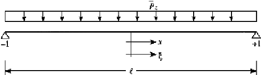
EXAMPLE 6.14 Simply Supported Beam
As an example of the mixed method, consider the solution of a simple beam on end supports
(Fig. 6.45). Let the whole beam be represented by a single element.
The state vector is
VM
]
T
z
=
[
wθ
(1)
The
CB
generalized variational form for a beam was developed in Chapter 2, Example 2.11,
Eq. (7). If the boundary terms are assumed to be satisfied at the outset,
+
,
00
x
d
0
w
θ
·
V
M
p
z
0
·
0
0
"
L
0
δ
00
1
x
d
z
T
···
···
−
dx
=
0
(2)
-
#
1
k
s
GA
d
x
1
−
0
1
EI
0
d
x
0
−
z
The beam element of Fig. 6.45 is of length
, beginning at
x
=−
/
2 and ending at
x
=+
/
2.
To express the axial coordinate in nondimensional form, define
ξ
=
2
x
/
. Then the element
is defined in the range
−
1
≤
ξ
≤
1
.
Also, note that
d
x
=
(
2
/)
d
. In terms of the coordinate
ξ
ξ
, (2) becomes
+
,
w
V
M
p
z
0
0
0
0
0
d
(
2
/)
0
"
ξ
x
δ
−
0
0
1
d
(
2
/)
ξ
z
T
dx
=
0
(3)
(
2
/)
d
1
−
1
/
k
s
GA
0
-
#
ξ
0
(
2
/)
d
ξ
0
−
1
/
EI
To justify ignoring the boundary terms in (2), choose trial functions for both displacements
and forces that satisfy the boundary conditions
(w
=
M
=
0at
ξ
=±
1
).
w
V
M
N
w
θ
V
M
w
θ
V
M
2
1
−
ξ
w
N
ξ
θ
=
=
(4)
ξ
N
V
−
ξ
2
1
N
M
z
z
FIGURE 6.45
Notation for Example 6.14.


Search WWH ::

Custom Search