The Finite Element Method - Mechanics of Structures: Variational and Computational Methods - page 406

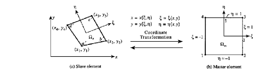
FIGURE 6.39
Isoparametric coordinate transformation.

The basic principle of isoparametric elements is that the interpolation functions for the
displacements are also used to represent the geometry of the element. For a four-sided
element, suppose the displacements u x ,u y in the global x, y directions are expressed as

4 4

u x = N i u xi , u u = N i u yi (6.129)

i = 1 i = 1

in which N i are the interpolation functions, and u xi ,u yi are the displacements at the nodes.
For an isoparametric element, the geometry of the element would be represented by the
same interpolation functions N i , i.e., the global coordinate values x, y of any point in the
element are

4 4

x = N i x i , y = N i y i (6.130)

i = 1 i = 1

where x i and y i are the coordinates of the i th node in the global coordinate system.
The concept of an isoparametric element is quite useful because it can facilitate an accu-
rate representation of irregular domains. However, the use of an isoparametric element can
make it difficult to perform the integration necessary to form the element stiffness matrix
and loading vector in terms of the global coordinates x and y because of the irregular shape
of the element. The irregular-shaped element can be visualized as a distortion of the corre-
sponding regular shaped element, such as the situation shown in Fig. 6.39. The integration
for the element in Fig. 6.39a can be transformed to the integration in the element of Fig.
6.39b, which is much easier to implement. To do so, it is necessary to build a relationship
or mapping between this distorted isoparametric element, called a slave element, and the
corresponding regular shaped element, called a parent or master element. The finite element
model is formed of the slave elements.
Consider the two-dimensional case shown in Fig. 6.39. The master element is

m , and the

slave element is

e . The local coordinate systems

(ξ , η) for these two elements have their

origins at the centroids of the elements, with ξ , η varying from − 1 to 1 as shown in Fig. 6.39.

The coordinate transformation will map the point (ξ , η) in the master element to x (ξ , η)

and y (ξ , η) in the slave element. From Example 6.9, Eq. (3), the interpolation functions are

given by

1
4 (

1
4 (

N 1 = 1 − ξ)( 1 − η) , = 1 + ξ)( 1 − η)

2

(6.131)

1
4 (

1
4 (

N 3 = 1 + ξ)( 1 + η) , = 1 − ξ)( 1 + η)

4