Information Technology Reference
In-Depth Information
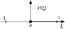
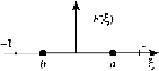
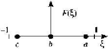
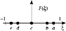
TABLE 6.7
Gaussian Quadrature Formulas
Gaussian Quadrature of
F
(ξ )
over the interval [
−
1
,
1]:
1
−
ξ
=
i
W
(
n
)
i
1
F
(ξ )
d
F
(ξ
i
)
n
=
Number of integration points
W
(
n
)
i
n
Configuration
Locations
ξ
i
Error
R
n
1
3
F
(
2
)
(
1
a
0
2
r
)
∗
√
1
135
F
(
4
)
(
1
2
a
/
3
1
r
)
−
√
1
b
/
3
1
√
3
a
/
5
5/9
15750
F
(
6
)
(
1
3
b
0
8/9
r
)
−
√
3
/
c
5
5/9
a
0.86113 63116
...
0.34785 48451
...
4
b
0.33998 10436
...
0.65214 51549
...
3472875
F
(
8
)
(
1
c
−
0.33998 10436
...
0.65214 51549
...
r
)
d
−
0.86113 63116
...
0.34785 48451
...
a
0.90617 98459
...
0.23692 68851
...
b
0.53846 93101
...
0.47862 86705
...
128
225
1
10
9
F
(
10
)
(
5
c
0
r
)
1
.
2377
×
d
−
0.53846 93101
...
0.47862 86705
...
e
−
0.90617 98459
...
0.23692 68851
...
F
(
n
)
(
∗
r
)
is the
n
th derivative with respect to
ξ
and
r
is a point in [
−
1
,
1].
The
n
Gauss integration points of Eq. (6.123) are found by solving
P
n
(ξ )
=
0 for its roots
ξ
i
,i
=
0
,
1
,
...
,n
−
1
.
The weighting functions are given by
(
−
ξ
i
)
2
1
W
(
n
)
i
=
=
...
i
1
,
2
,
,n
(6.124)
]
2
[
nP
n
−
1
(ξ
)
i
Gaussian quadrature is the most frequently used integration procedure in finite element
calculations because for the same number of integration points, the accuracy is better than
that of the Newton-Cotes method.
EXAMPLE 6.11 Determination of Integration Points and Weighting Coefficients
Establish the integration points and weighting coefficients for Gaussian quadrature in the
domain [
.
First find the integration points. For
n
−
1
,
1] if
n
=
2
=
χ(ξ)
=
(ξ
−
ξ
)(ξ
−
ξ
).
2
,
Use Eq.(6.123)
1
2
1
1
1
(ξ
−
ξ
)(ξ
−
ξ
)
d
ξ
=
0
,
1
(ξ
−
ξ
)(ξ
−
ξ
)ξ
d
ξ
=
0
(1)
1
2
1
2
−
−
Upon integration, it follows that
ξ
ξ
=−
/
ξ
+
ξ
=
1
3
,
0
(2)
1
2
1
2


Search WWH ::

Custom Search