Information Technology Reference
In-Depth Information
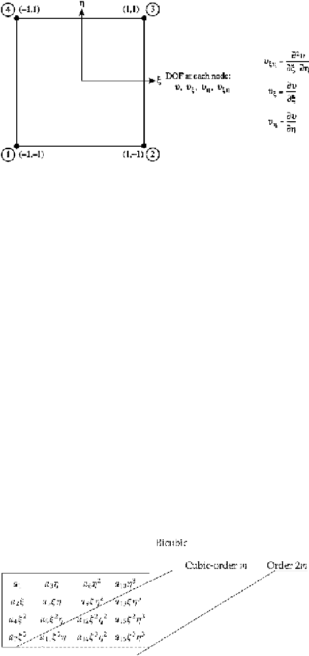
FIGURE 6.35
A rectangular element.
so that
2
3
N
1
=
1
−
3
ξ
+
2
ξ
.
In a similar fashion, the remaining interpolation functions
N
2
,N
3
,
and
N
4
of Figs. 6.34c, d,
and e are found to be
2
,
2
3
,
2
N
2
=−
ξ(ξ
−
1
)
=
3
ξ
−
2
ξ
4
=−
ξ
(ξ
−
1
)
3
These are referred to as Hermitian polynomials. The deflection trial function then becomes
2
3
2
2
3
2
w(ξ)
=
(
1
−
3
ξ
+
2
ξ
)w
a
−
ξ(ξ
−
1
)
θ
a
+
(
3
ξ
−
2
ξ
)w
b
−
ξ
(ξ
−
1
) θ
b
which corresponds to Chapter 4, Eq. (4.47b).
Two-Dimensional Case in Cartesian Coordinates
The two-dimensional Hermitian case follows closely the development of the two-dimen-
sional Lagrangian interpolation. A trial function for the rectangular of Fig. 6.35 would be
=
v
v
η
1
v
v
η
4
N
1
η
N
2
η
N
3
η
N
2
η
1
4
v
ξ
1
v
ξη
1
v
ξ
4
v
ξη
4
N
T
ξ
u
=
[
N
1
ξ
N
2
ξ
N
3
ξ
N
4
ξ
]
RN
η
(6.89)
v
v
η
2
v
v
η
3
2
3
v
ξ
2
v
ξη
2
v
ξ
3
v
ξη
3
The corresponding polynomial contains 16 terms and is a bicubic expansion, i.e., it is formed
by the multiplication of two one-dimensional cubic polynomials.
(6.90)


Search WWH ::

Custom Search