Information Technology Reference
In-Depth Information
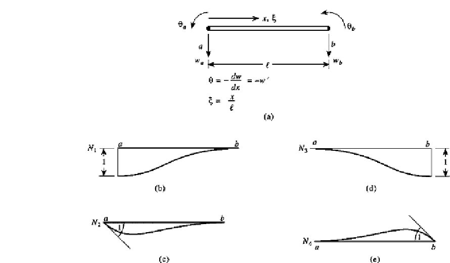
FIGURE 6.34
A beam element.
The superscripts of
v
denote the order of differentiation, and the subscripts refer to the end
points. Also,
k
=
(
j
−
1
)
m
+
i
. Similar to the Lagrangian case [Eqs. (6.62) and (6.63)],
N
k
must satisfy
1
d
i
−
1
N
k
(ξ )
d
when
ξ
=
ξ
(
k
=
(
j
−
1
)
m
+
i
)
j
=
(6.87)
ξ
i
−
1
0
when
ξ
=
ξ
(
k
=
(
j
−
1
)
m
+
i
)
j
It is assumed that 2
m
conditions are available for constructing each of the 2
m
interpolation
functions
N
i
. Choose a polynomial series of order 2
m
−
1 with 2
m
coefficients
u
2
m
ξ
(
2
m
−
1
)
(6.88)
A particular
N
i
is developed to satisfy the requirements of Eq. (6.87). This procedure leads
to 2
m
equations for determining an interpolation function. A similar technique applies for
the case of multiple nodal points.
For the beam element of Fig. 6.34, the interpolation functions for the displacement are
derived in the same manner used to obtain Eq. (4.47b) of Chapter 4. Begin with the trial
solution
2
N
i
=
u
1
+
u
2
ξ
+
u
3
ξ
+···+
2
3
.
w(ξ)
=
N
1
w
+
N
2
θ
+
N
3
w
+
N
4
θ
b
and polynomial
N
i
=
u
1
+
u
2
ξ
+
u
3
ξ
+
u
4
ξ
a
a
b
To determine
N
1
, which should appear as shown in Fig. 6.34b, apply the conditions
w(
0
)
=
=−
w
(
=−
w
(
w
=
1
,
θ(
0
)
=
θ
0
)
=
0
,
w(
1
)
=
w
=
0, and
θ(
1
)
=
θ
1
)
=
0, giving
a
a
b
b
=
ξ
=
0
N
1
=
1
w(
0
)
=
1
u
1
N
1
=
=
ξ
=
0
0
θ(
0
)
=
0
u
2
/
=
+
+
+
ξ
=
1
N
1
=
0
w(
1
)
=
0
u
1
u
2
u
3
u
4
N
1
=
=
(
ξ
=
1
0
θ(
1
)
=
0
u
2
+
2
u
3
+
3
u
4
)/
Note that these conditions are given in Eq. (6.87). The relations on the right-hand side can
be solved to give
=
=
=−
=
u
1
1
u
2
0
u
3
3
u
4
2


Search WWH ::

Custom Search