The Finite Element Method - Mechanics of Structures: Variational and Computational Methods - page 381

and

N 1 ξ N 1 η = ( 1 − ξ)( 1 − η)

N 2 ξ N 1 η = ξ( 1 − η)

(5)

N 2 ξ N 2 η = ξη
N 1 ξ N 2 η = ( 1 − ξ)η

Then u x can be written as

u x 1
u x 2
u x 3
u x 4

=

u x = [ ( 1 − ξ)( 1 − η) ξ( 1 − η) ξη ( 1 − ξ)η ] N x v x (6)

Note that N x here is the same as that in Eq. (6.18).

Lagrangian Elements
The Lagrange family of elements is characterized by the nodal unknowns being values of the
dependent variables. This is in contrast to the Hermitian element , e.g., beam element, which
includes also the derivatives (slopes) of the displacement (deflection) among the unknown
nodal parameters. With the exception of some lower order members of the family, the La-
grange elements have internal nodes. This is sometimes considered to be disadvantageous.
Elements with all nodes on the boundary are often referred to as serendipity elements .

One-Dimensional Case in Natural Coordinates
An interesting means of expressing coordinates is by using so-called natural (or homoge-
neous ) coordinates . These coordinates are a mapping of physical coordinates into nondimen-
sional coordinates that assume the values one or zero at the nodes. Natural coordinates are
commonly used to create an interpolation function and nodal pattern for two-dimensional
elements. We begin the study of natural coordinates by defining them for a single dimension.
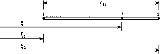
For the one-dimensional case, consider a line with points 1, 2, and i defined by coordinates

ξ 1 , , respectively, as shown in Fig. 6.28. The natural coordinates L 2 and L 1 , which

serve as weighting functions, are defined by the ratios

ξ 2 , and ξ

= ξ − ξ = (ξ

− ξ ) − (ξ − ξ )

= ξ

− ξ
ξ 2 − ξ 1

1
ξ 2 − ξ 1

2 1 1 2

L 2 L 1 (6.66)

ξ 2 − ξ 1

where

1 is the distance to point i . Note that the natural coordinates are not independent,
since they have been nondimensionalized, so that

ξ − ξ

L 1 + L 2 = 1 (6.67)

FIGURE 6.28
One-dimensional natural coordinates L 1 and L 2 .