The Finite Element Method - Mechanics of Structures: Variational and Computational Methods - page 377

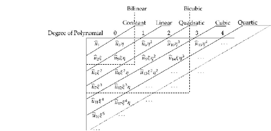
Note, for example, from Eq. (6.61) or the Pascal triangle, that ten terms are needed to form
a complete two-dimensional cubic polynomial.
There are several procedures available for using interpolation polynomials to represent
the response throughout a two- or three-dimensional element and to place a network of
nodes on the element. Three schemes—Lagrangian interpolation, natural coordinates, and
Hermitian interpolation—are considered in this section. Each is introduced as a unidirec-
tional polynomial and then extended to the multidimensional case.

6.5.6 Lagrangian Interpolation

In order to study the problem of creating an interpolation trial function for two- and three-
dimensional elements, we begin by considering a one-dimensional Lagrange polynomial
which provides an interpolation function for a line divided into segments. Products of these
polynomials lead to interpolation functions, along with a network of nodes, for multidi-
mensional elements.

One-Dimensional Case in Cartesian Coordinates
Consider a line (Fig. 6.26) divided into segments of equal length by m points (nodes), with
the nodes defined by the coordinates

ξ 1 , ξ 2 , ... , ξ m . We wish to establish a function u (ξ )

that takes on the exact displacements v m at these m points and also provides

approximate displacement values at points intermediate to these nodal points. In the case
of Lagrangian interpolation, a polynomial u

v 1 , v 2 , ... ,

(ξ ) of order m − 1isdefined to replace the true

displacements such that u (ξ ) is equal to v

i at the nodal points

ξ

i , i.e., i

(ξ ) = v = ...

u

i ,

i 1 , 2 , ,m

i

Express u (ξ ) as

m m

u (ξ ) = N i (ξ ) u (ξ ) = N i v i = 1 , 2 , ... ,m (6.62)

i i

i i