Structural Analysis Methods I: Beam Elements - Mechanics of Structures: Variational and Computational Methods - page 200

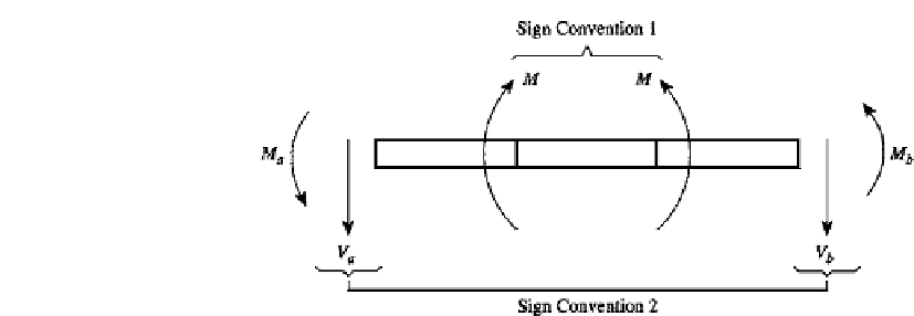
FIGURE 4.9
A beam element with positive internal bending moment M (Sign Convention 1) and nodal moments and shear
forces (Sign Convention 2).

Evaluation of the Stiffness Matrix Using the Principle of Virtual Work
The purpose of this section on the use of a trial series is to show how the principle of
virtual work can be employed to evaluate an element stiffness matrix. This is a very general
procedure which can be used to derive stiffness matrices for any element. Recall from
Chapter 2 that for kinematically admissible virtual displacements, the principle of virtual
work relation

− δ − δ =

0 assures that the system is in equilibrium.
For a beam element with no consideration of either axial or shear deformation effects, the
element contribution to the principle can be written in terms of the operator k D as (Chapter
2, Example 2.7)

W i W e

b
a δw

b
a δw

k D

w dx − p z dx (4.52)

with k D

x d 2 EI d x and p z is the applied loading intensity along the beam. The
bar over p z ind icate s t hat this is a prescribed or app lied qu antity. It is possible to include
the term

k D

= =

] a in Eq. (4.52), where M and V are concentrated loads on the
ends a, b of the element. Howe ve r, it is assumed here that applied loads on the boundary

− [ M δθ + V δw

are included in the term b
a

δw .

Also, a derivative with a subscript on the left side,
e.g., x d, means that the derivative is taken on the preceeding variable. Thus,

p z dx

δw

x d is the

d
dx

same as . The trial series satisfies the displacement boundary conditions. Then Eq.

(4.52) is the element contribution to the satisfaction of the conditions of equilibrium for the
whole system. Since the assumed displacement series is approximate, an “approximate”
fulfillment of equilibrium should be expected.
The variational quantities

δw

δw expressed in terms of the trial series are needed
to proceed with Eq. (4.52). Note that in Eq. (4.46a), v contains unknown discrete values of
displacements, G contains constant factors for the polynomials, and only N u is a function
of the axial coordinate x . Then

δw and

v T G T N u = δ v T N T

δw = δ( N u Gv ) = N u G δ v = δ (4.53)

v T contains the virtual end displacements. Also, set N u =

where N = N u G and δ B u =

[0026 x ] and form

w = N u Gv N v = B u Gv = = Bv

(4.54)

δw =

v T B T

δ = δ

B v