Information Technology Reference
In-Depth Information
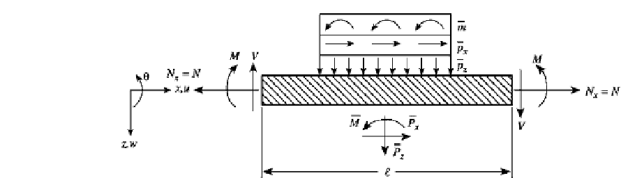
FIGURE 2.3
Positive state variables
(
u,
w
,
θ
,M,V,N
)
and positive applied loadings (variables with superscript bars) for a
beam.
EXAMPLE 2.1 Beam Theory
Consider the use of Eq. (2.9) to calculate the strain energy in a beam with an internal axial
force and bending moment.
For the engineering beam theory of Chapter 1, it is assumed that the deformations are
small, the material obeys Hooke's law, and the length of the beam is much greater than
the cross-sectional dimensions, e.g., width and depth. All of the state variables of the beam
are referred to the beam axis (the centroid), so that we are dealing with a one-dimensional
problem. The positive directions of applied loadings and state variables are indicated in
Fig. 2.3. For the Euler-Bernoulli beam theory, in which shear deformation effects are not
taken into account, the only non-zero strain is
x
. Thus,
V
1
2
1
2
T
E
dV
U
i
=
=
x
E
x
dV
(1)
V
As indicated in Chapter 1, the use of Bernoulli's hypothesis on the cross-section leads to
[Chapter 1, Eq. (1.98)]
u
=
u
0
(
x
)
+
z
θ
and
θ
=−
d
w/
dx
,
z
d
2
du
dx
=
du
0
dx
−
w
dx
2
=
(2)
x
dA dx
and since by definition
A
zdA
=
=
With
dV
0 if the quantities are referred to the
centroid, for a beam of length L, the strain energy of (1) reduces to
E
du
0
dx
2
2
L
z
d
2
1
2
1
2
w
U
i
=
V
x
E
x
dV
=
dx
−
dA dx
0
A
EA
du
0
dx
2
E
d
2
dx
2
2
z
2
dA
dx
L
1
2
w
=
+
0
A
EA
2
dx
2
2
dx
L
du
0
dx
2
d
2
EI
2
w
=
+
(3)
0
This final expression can also be written in terms of internal forces, leading to the expres-
sion for the complementary potential energy. From Chapter 1, Eq. (1.125),
EI
d
2
dx
2
(
w/
)
=
−
M
. For the axial extension of the centerline of the beam (Chapter 1, Eq. 1.106a),
x
|
axial
=
0
x
=
du
0
/
dx
or
N
=
EA
0
x
=
EA
(
du
0
/
dx
)
. Thus, (3) becomes
L
N
2
EA
+
dx
M
2
EI
1
2
U
i
=
(4)
0


Search WWH ::

Custom Search