Computational fluid dynamics: applications in pharmaceutical technology - Computer-Aided Applications in Pharmaceutical Technology - page 238

variable at a given point can be expressed as a function of the value at a
neighboring point and its change due to the shift of Δx (Blazek, 2005;
Sayma, 2009).
The fi nite element method , as a method for solving partial differential
equations, was developed between 1940 and 1960, and its application
was later extended to fl uid fl ow problems. Unlike the fi nite difference
method, the fi nite element method can be applied in problems with
complex geometry and unstructured grids of various shapes. The distinct
difference between these methods is that the fi nite difference method
requires only the values of the variables at grid nodes, without information
about behavior between the nodes, while the fi nite element method takes
into account variations within each element. The fi nite element method
involves discretization of computational domain and discretization of
differential equations. Discretization of the spatial domain considers its
subdivision into non-overlapping elements of various shapes. In two-
dimensional problems, triangular or rectangular elements are commonly
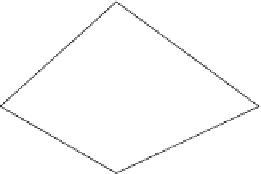
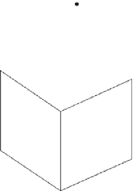
used, while the most common element types for three-dimensional
problems are the tetrahedral, hexahedral, and prismatic elements
(Figure 7.2). Each element is formed by connecting a number of nodes/

￿

￿ ￿

Example of: (a) triangular; (b) tetrahedral; and
(c) prismatic element

Figure 7.2