Noise-induced phenomena in zero-dimensional systems - Noise-induced Phenomena in the Environmental Sciences - page 80

V φ

0.4

0.2

2 φ 2 1 1

0.2

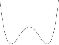
Figure 3.17. Typical shape of a bistable potential. In particular, the figure refers to
V

4 2

= φ / 4 − φ / 2; the minima are at φ m , 1 =− 1 and φ m , 2 = 1, and the height of the

potential barrier, situated at φ b = 0, is V = 1 / 4.

Figure 3.17 shows an example of bistable potential, with the two minima, φ m , 1 and

φ m , 2 , separated by a potential barrier of height V , situated at φ = φ b . In this case the

4 2

potential is V ( φ ) = φ / 4 − φ / 2. In the absence of stochastic and periodic forcings,

the dynamics of the variable φ are described by

d d t =− d V

d

2 )

= φ (1 − φ . (3.57)

φ

Depending on the initial condition, the system will tend to either one of the two
stable states (see Fig. 3.18 ) associated with the minima

φ m of the potential (i.e.,

φ m , 1 =− 1 in this example). The dynamics within each potential well

are characterized by the time scale typical of the process close to the minimum; this
time scale is proportional to

1and φ m , 2 =

d 2 V
d

− 1

φ = φ m

=

t iw (3.58)

φ

2

and can be assumed as the intrawell relaxation time. In example ( 3.57 )wefind
t iw = 1 / 2.

2 φ

t

1.5

1

0.5

t

0.5 1 1.5 2 2.5 3

0.5

1

1.5

2

Figure 3.18. Examples of time trajectory for nonforced dynamics regulated by
Eq. ( 3.57 ). The different curves correspond to different initial conditions.