Environmental Engineering Reference
In-Depth Information
q
t
1
0.8
0.6
0.4
0.2
t
0.2
(a)
ξ
dn
t
0.5
t
0.5
1
(b)
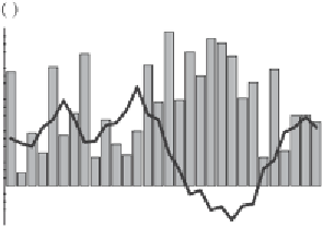
Figure 2.7. Example of the relations among (a) the external forcing
q
(
t
) (gray bars),
the threshold
θ
(continuous line), and (b) the corresponding DMN.
cases are considered by
Masoliver andWeiss
,
1994
;
Christophorov
,
1996
;and
Julicher
et al.
,
1997
), the presence of the state dependency in
k
1
and
k
2
profoundly affects the
dynamics of
φ
because of the modification of the distribution of the residence times
in states
2
[Fig.
2.7
(b)]. The fact that this distribution is not exponential as
in the case of the standard DMN is consistent with a general property of processes
with state-dependent rates (
Daly and Porporato
,
2006
,
2007
).
When transition rates
k
1
and
k
2
depend on the state of the system, the process
remains analytically solvable. In fact, the steps leading to steady-state solution (
2.31
)
are not affected by a possible state dependency of the transition rates. As a conse-
quence, we simply obtain the solution in the state-dependent case from Eq. (
2.31
)by
setting
k
1
=
1
and
k
1
(
φ
)and
k
2
=
k
2
(
φ
):
C
1
f
1
(
exp
k
1
(
d
φ
φ
)
f
1
(
φ
)
f
2
(
1
f
2
(
k
2
(
p
(
φ
)
=
)
−
−
φ
)
+
,
(2.44)
φ
)
φ
φ
)
φ
where
C
is a normalization constant we calculate by imposing the condition that the
integral of
p
(
φ
) in the domain of the definition of
φ
be equal to 1. The zeros of
f
1
(
φ
)
and
f
2
(
) are the natural boundaries for the dynamics and represent the limits of the
domain of
φ
φ
(see also
Bena
,
2006
). An alternative representation of the pdf, which is


Search WWH ::

Custom Search