Deterministic mechanisms of pattern formation - Noise-induced Phenomena in the Environmental Sciences - page 281

ω Z

′ −

r

r

Z

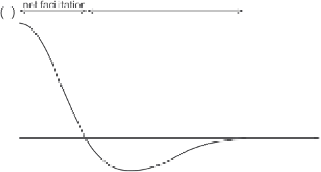
Figure B.3. Typical kernel that exhibits local activation-long-range inhibition.

Fig. B.3 can be obtained for example as the difference between two exponential
functions of the form

= b 1 exp

2

− b 2 exp

2

z
q 1

z
q 2

ω ( z ) − − , (B.13)

where 0 < q 1 < q 2 and b 1 and b 2 are two coefficients expressing the relative im-

portance of the facilitation and competition components of the kernel (see also
Chapter 6).
The dynamics expressed by Eq. ( B.12 ) may lead to pattern formation through
mechanisms that resemble those of Turing's instability. In fact, patterns emerge as a
result of the spatial interactions, which destabilize the uniform stable state φ 0 of the

local dynamics. To study the stability of the state φ = φ 0 with respect to infinitesimal

perturbations, we linearize Eq. ( B.12 ) around the steady state φ = φ 0 . Indicating by

ˆ

φ = φ − φ 0 the amplitude of the (“small”) perturbation, we obtain
∂

ˆ

φ
∂

ˆ

) ˆ

f ( r − ( r , t )d r , = φ φ 0 ) +

ω

( | r | φ (B.14)

t

where f ( φ = φ 0 .

Solutions of Eq. ( B.14 ) can be expressed in the form of integral sums of the
harmonics ˆ

φ 0 ) is the derivative of the function f ( φ ), calculated for

φ ( r , t ) ∝ exp[ γ t + i k · r ], where each harmonic is a solution of ( B.14 ),

k = ( k x , k y ) is the wave-number vector, and the growth factor γ is an eigenvalue of

r − Eq. ( B.14 ). Substituting this solution into Eq. ( B.14 ), setting z , and cancel-

ing out the exponential function, we obtain the dispersion relation, that is, the relation
between k and

=| r |

γ in solutions of ( B.12 ) obtained as small perturbations of the state

φ = φ 0 :

f ( f ( γ ( k ) = φ 0 ) +

ω

( z )exp[ i k · z ]d z = φ 0 ) + W ( k ) , (B.15)