Environmental Engineering Reference
In-Depth Information
a
b
ξ
dn
t
ξ
dn
t
1
0.5
0.5
t
t
0.5
0.5
1
1
φ
t
φ
t
12
0.8
10
0.6
8
6
0.4
4
0.2
2
10 15 20 25 30 35
t
t
5
10
20
30
c
d
ξ
dn
t
ξ
dn
t
0.4
0.75
0.2
0.5
0.25
t
t
0.2
0.25
0.5
0.4
1
φ
t
φ
t
1.4
0.8
1.2
0.6
0.4
35
t
5
10
15
20
25
30
0.2
0.8
t
0.6
5
10
15
20
25
30
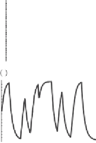
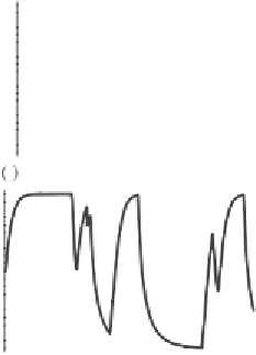
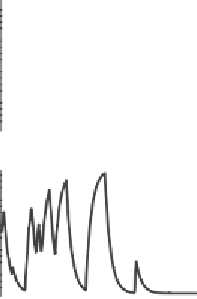
Figure 2.3. The four panels (a)-(d) show the noise path and the corresponding
evolution of the
(
t
) variable from Eq. (
2.16
): (a) Example 2.1, Example 2.2,
(c) Example 2.3, (d) Example 2.4.
φ
Example 2.3:
φ
(
t
) increases following a (shifted) logistic law (see Subsection
3.2.1.1
) when
the noise is in the
1
state, whereas it decreases exponentially in the
2
state:
f
1
(
φ
)
=
(
φ
−
a
)(1
−
φ
)
,
f
2
(
φ
)
=−
φ,
(2.19)
where
a
is a constant. An example for
a
=−
0
.
5 is shown in Fig.
2.3
(c).


Search WWH ::

Custom Search